Computer vision
The Beginner’s Guide to Semantic Segmentation
15 min read
—
Sep 16, 2021
Semantic Segmentation is the task of assigning a class label to every pixel in the image. Read this guide to explore the most common approaches to Semantic Segmentation and its real-world applications.

Guest Author and Founder
What is in this image, and where in the image is it located?
Semantic Segmentation is what can help you answer this question.
And—
We are about to walk you through it.
As you might already know, Image Segmentation techniques can be classified into three groups, depending on the amount and type of information they convey:
Semantic Segmentation
Instance Segmentation
Panoptic Segmentation
Pro tip: You can check out this Simple Guide to Image Segmentation to learn more.
The purpose of this article, however, is to get you started with Semantic Segmentation.
We will provide you with all the information (and tools!) you need.
Here’s what we’ll cover:
What is Semantic Segmentation?
Semantic Segmentation Deep Learning methods
Loss functions
Real-world applications of Semantic Segmentation
Ready to streamline AI product deployment right away? Check out:
What is Semantic Segmentation?
Semantic Segmentation follows three steps:
Classifying: Classifying a certain object in the image.
Localizing: Finding the object and drawing a bounding box around it.
Segmentation: Grouping the pixels in a localized image by creating a segmentation mask.
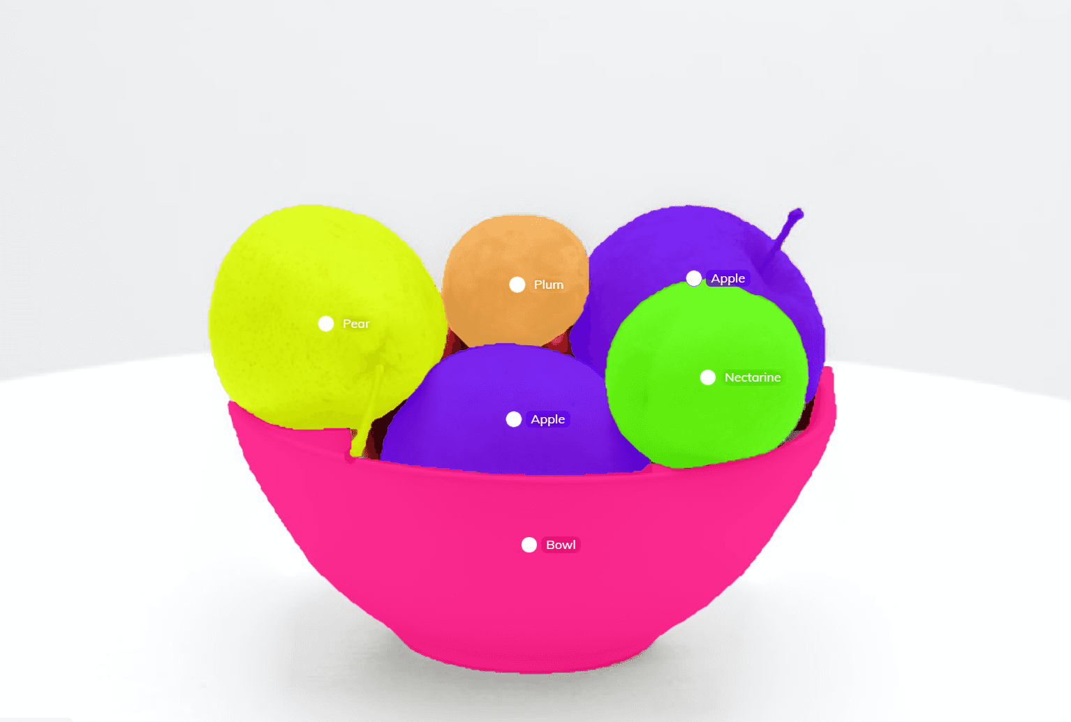
Essentially, the task of Semantic Segmentation can be referred to as classifying a certain class of image and separating it from the rest of the image classes by overlaying it with a segmentation mask.
It can also be thought of as the classification of images at a pixel level.
Below is an example of how you can perform semantic segmentation using V7.
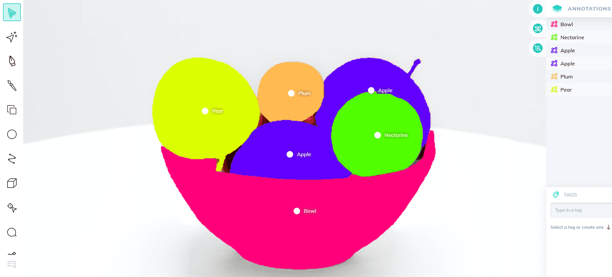
Semantic Segmentation in V7
The goal is simply to take an image and generate an output such that it contains a segmentation map where the pixel value (from 0 to 255) of the iput image is transformed into a class label value (0, 1, 2, … n).
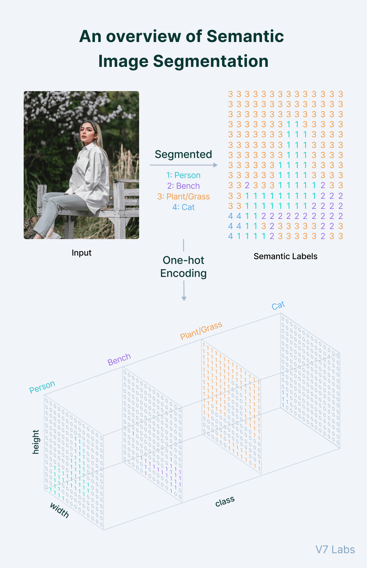
An overview of the Semantic Image Segmentation process
Pro Tip: Looking for the perfect data annotation tool to perform Semantic Segmentation? See this list of 13 Best Image Annotation Tools.
Now, let’s explore deep learning methods for semantic segmentation.
Semantic Segmentation Deep Learning methods
Semantic Segmentation often requires the extraction of features and representations, which can derive meaningful correlation of the input image, essentially removing the noise.
Pro Tip: Read A Simple Guide to Data Preprocessing in Machine Learning to learn more about data preparation
The convolutional neural network (CNN) performs this task and is frequently used in most computer vision tasks.
The following section will explore the different semantic segmentation methods that use CNN as the core architecture. The architecture is sometimes modified by adding extra layers and features, or changing its architectural design altogether.
Fully Convolutional Network
CNN consists of a convolutional layer, a pooling layer, and a non-linear activation function.
Pro Tip: Check out 12 Types of Neural Network Activation Functions: How to Choose?
In most cases, CNN has a fully connected layer at the end in order to make class label predictions.

CNN with fully connected layer
But—
When it comes to semantic segmentation, we usually don’t require a fully connected layer at the end because our goal isn’t to predict the class label of the image.
In semantic segmentation, our aim is to extract features before using them to separate the image into multiple segments.
However, the issue with convolutional networks is that the size of the image is reduced as it passes through the network because of the max-pooling layers.
To efficiently separate the image into multiple segments, we need to upsample it using an interpolation technique, which is achieved using deconvolutional layers.

CNN with upsampling and deconvolutional layer
In general AI terminology, the convolutional network that is used to extract features is called an encoder. The encoder also downsamples the image, while the convolutional network that is used for upsampling is called a decoder.
Here’s a visual representation of convolutional encoder-decoder.
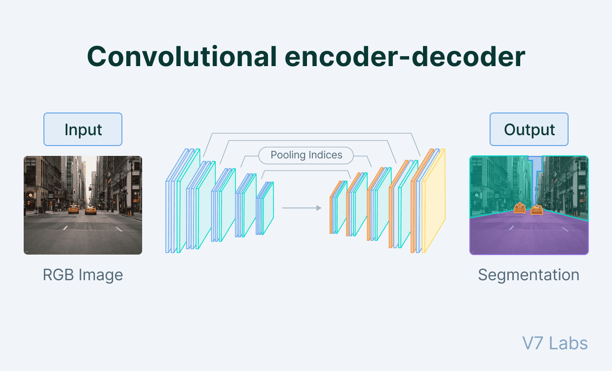
Convolutional encoder-decoder structure
The output yielded by the decoder is rough, because of the information lost at the final convolution layer i.e., the 1 X 1 convolutional network. This makes it very difficult for the network to do upsampling by using this little information.
To address this upsampling issue, the researchers proposed two architectures: FCN-16 and FCN-8.
In FCN-16, information from the previous pooling layer is used along with the final feature map to generate segmentation maps. FCN-8 tries to make it even better by including information from one more previous pooling layer.
Pro Tip: Learn more about data compression from our Beginner's Guide to Autoencoders.
U-net
The U-net was a modification of a fully convolutional network.
It was introduced by Olaf Ronneberger et al. in 2015 for medical purposes—primarily to find tumors in the lungs and brain.
The U-net has a similar design of an encoder and a decoder.
The former is used to extract features by downsampling, while the latter is used for upsampling the extracted features using the deconvolutional layers. The only difference between the FCN and U-net is that the FCN uses the final extracted features to upsample, while U-net uses something called a shortcut connection to do that.
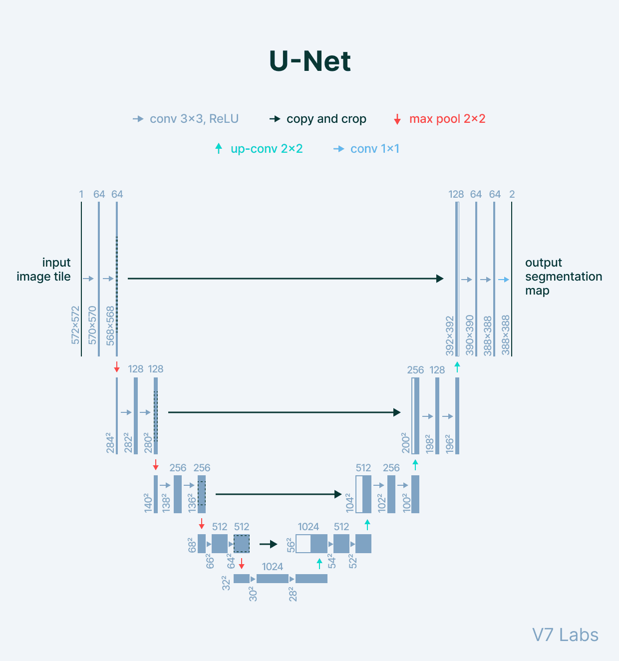
U-net architecture
The shortcut connection in the U-Net is designed to tackle the information loss problem.
Pro tip: Ready to train your models? Have a look at Mean Average Precision (mAP) Explained: Everything You Need to Know
The U-net is designed in such a manner that there are blocks of encoder and decoder. These blocks of encoder send their extracted features to its corresponding blocks of decoder, forming a U-net design.
So far, we have learned that as the image travels through the convolutional networks and its size is reduced.
This is because it simultaneously max-pools layers, which means that information is lost in the process. This architecture enables the network to capture finer information and retain more information by concatenating high-level features with low-level ones.
This process of concatenating the information from various blocks enables U-net to yield finer and more accurate results.
Pyramid Scene Parsing Network (PSPNet)
Pyramid Scene Parsing Network (PSPNet) was designed to get a complete understanding of the scene.
Scene parsing is difficult because we are trying to create a Semantic Segmentation for all the objects in the given image.
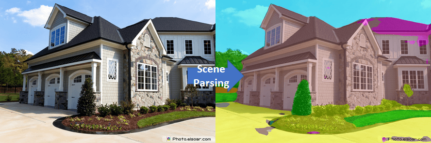
Scene Parsing
The FCN doesn’t perform too well because of the information loss that we discussed earlier.
Some of this information is lost because of the spatial similarities between two different objects. A network can capture spatial similarities if it can exploit the global context information of the scene.
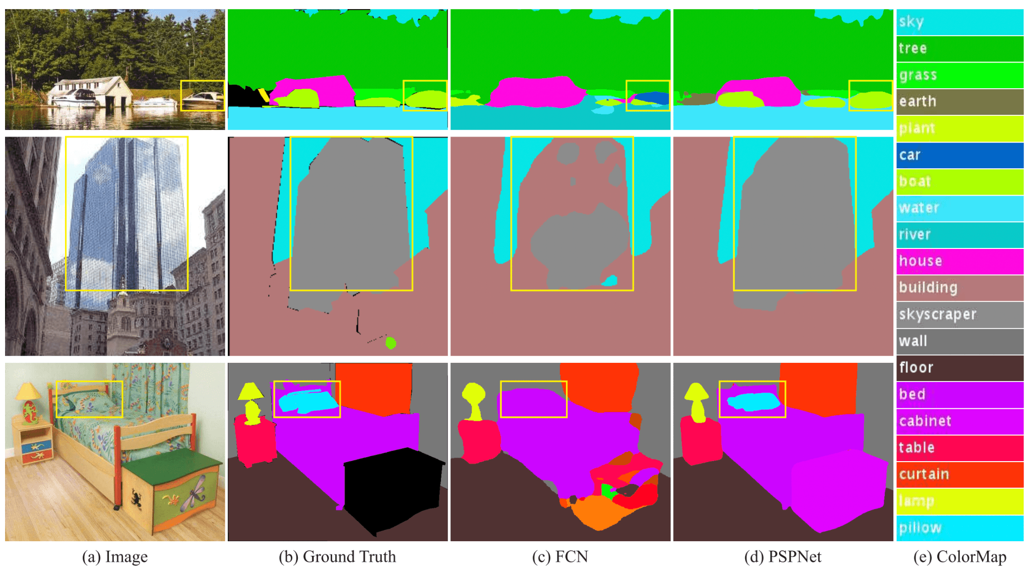
The comparison of FCN and PSPNet performance
PSPNet exploits the global context information of the scene by using a pyramid pooling module.

PSPNet with Pytaming Pooling Module
From the diagram above, we can see that the pyramid pooling module has four convolutional components.
The first component indicated in red yields a single bin output, while the other three separate the feature map into different sub-regions and form pooled representations for different locations.
These outputs are upsampled independently to the same size and then concatenated to form the final feature representation.
Because the filter size of the convolution network is varied (i.e., 1X1, 2X2, 3X3, and 6X6), the network can extract both local and global context information.
The concatenated upsampled result from the pyramid module is then passed through the CNN network to get a final prediction map.
DeepLab
Google developed DeepLab, which also uses CNN as its primary architecture.
Unlike U-net, which uses features from every convolutional block and then concatenates them with their corresponding deconvolutional block, DeepLab uses features yielded by the last convolutional block before upsampling it, similarly to CFN.
The Deeplab applies atrous convolution for upsampling.
Atrous convolution
Atrous convolution (or Dilated convolution) is a type of convolution with defined gaps.
To better understand it, let’s imagine k is the dilation rate.
If k=1, the convolution will be normal. But if we increase the value of k by one—for example, k=2—then we skip one pixel per input.
See the image below.
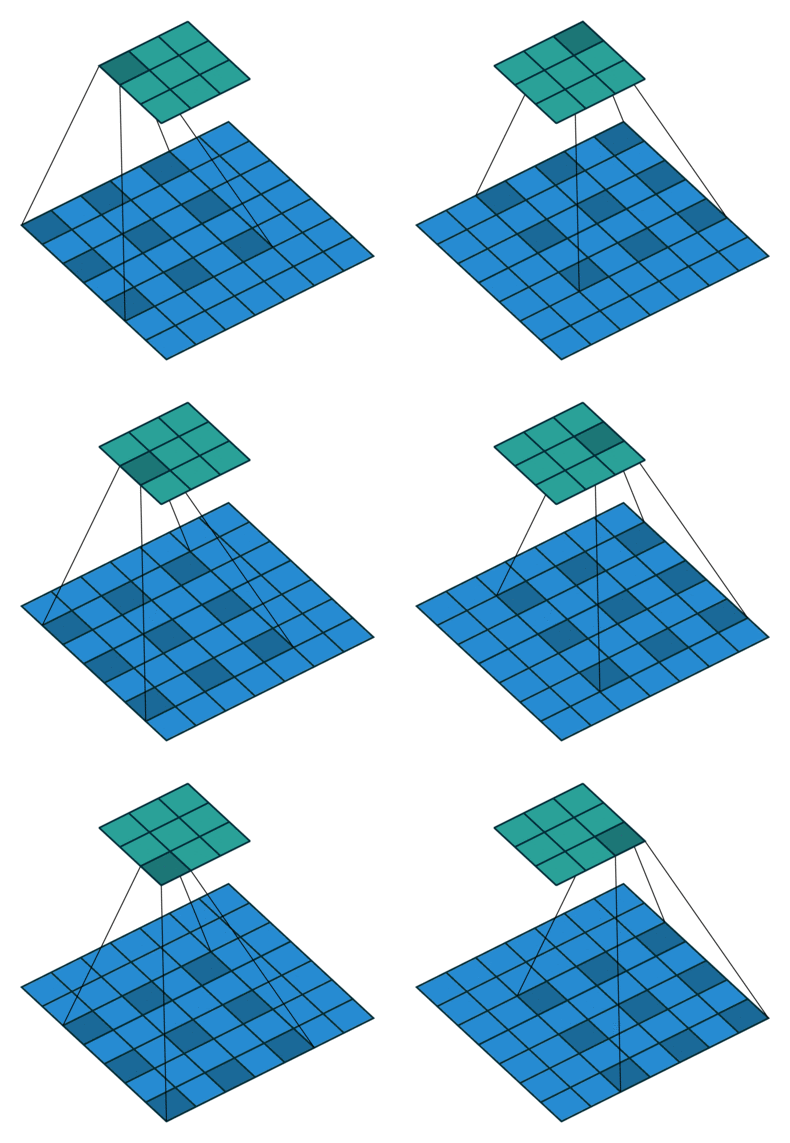
Dilated convolution
Dilation rate defines the spacing between the values in a convolution filter.
As shown in the image above, a 3x3 filter with a dilation rate of 2 will have the same field of view as a 5x5 filter while only using nine parameters.
The advantage of using an Atrous or Dilated convolution is that the computation cost is reduced while capturing more information.
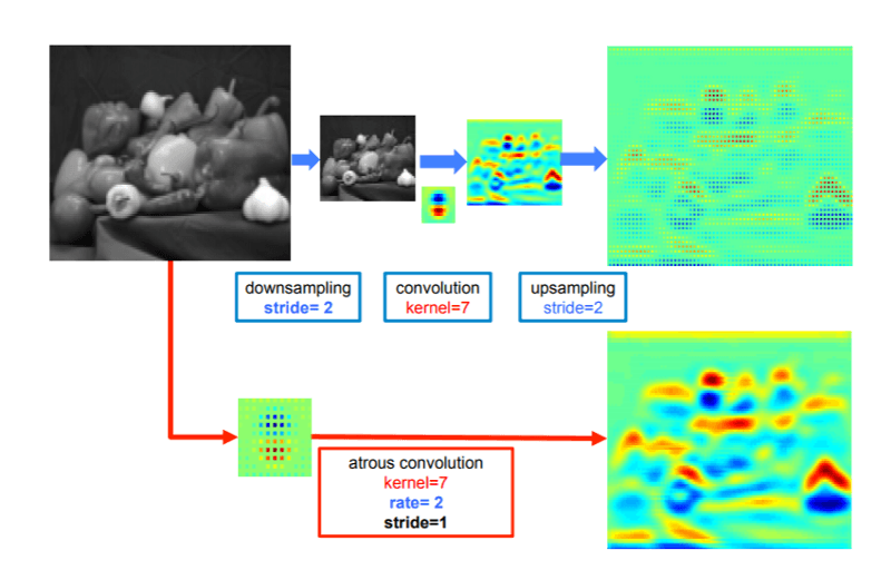
In the image above, the bottom figure shows that Atrous convolution achieves a denser representation than the top figure.
DeepLab V1
Now you know that DeepLab’s core idea was to introduce Atrous convolution to achieve denser representation where it uses a modified version of FCN for the task of Semantic Segmentation.
This idea introduced DeepLab V1 that solves two problems.
1. Feature resolution
The issue with DCNN is multiple pooling and down-sampling, which causes a significant reduction in spatial resolution.
To achieve a higher sampling rate, the down-sampling operator was removed from the last few max-pooling layers, and instead, up-sample the filters (atrous) in subsequent convolutional layers were added.
2. Localization accuracy due to DCNN invariance
In order to capture fine details, data scientists employed a fully connected Conditional Random Field (CRF), which smoothens and maximizes label agreement between similar pixels.
The CRF also enables the mode to create global contextual relationships between object classes.
DeepLab V2
DeepLab V1 was further improved to represent the object in multiple scales.
In the previous section, we saw how PSPNet used a pyramid pooling module to achieve multiple Semantic Segmentation with greater accuracy.
Building on that theory, DeepLab V2 used Atrous Spatial Pyramid Pooling (ASPP).
The idea was to apply multiple atrous convolutions with different sampling rates and concatenate them together to get greater accuracy.
DeepLab V3
The aim of DeepLab V3 was to capture sharper object boundaries.
This was achieved by adopting the encoder-decoder architecture with atrous convolution.
Here are the advantages of using encoder-decoder architecture:
It can capture sharp object boundaries.
It can capture high semantic information because the encoders gradually reduce the input image while extracting vital spatial information; similarly, decoders gradually recover spatial information.
ParseNet
ParseNet was introduced by Wei Liu et al. in 2015.
The authors of this paper suggested that FCN cannot represent global context information.
Contextual representation of the data or image is known to be very useful for improving performance segmentation tasks. Because FCN lacks contextual representation, they are not able to classify the image accurately.
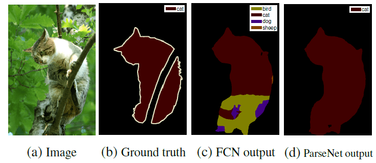
The comparison between FCN and ParseNet output
To acquire global context information or vector, the authors used a feature map that was pooled over the input image, i.e., global average pooling.
Once acquired, the global context vector was then appended to each of the features of the subsequent layers of the network.
It is worth noting that global context information can be extracted from any layer, including the last one.
The authors stated that:
The quality of Semantic Segmentation is greatly improved by adding the global feature to local feature map.
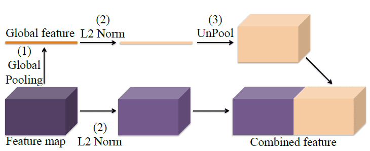
ParseNet contexture model
The image above represents the overview of the ParseNet contexture module.
As you can see, once the global context information is extracted from the feature map using global average pooling, L2 normalization is performed on them.
Similarly, L2 normalization is also performed directly on the feature map.
To combine the contextual features to the feature map, one needs to perform the unpooling operation. It ensures that both features are of the same size.
In conclusion, ParseNet performs better than FCN because of global contextual information.
Loss functions
Loss functions are important in all neural network-related tasks.
The loss function ensures that the neural network optimizes itself by reducing the error it generates during the training process.
Before we discuss the loss function, it is worth recalling that semantic segmentation is a classification task where the final result yields segmentation maps based on the class label.
Class labels vary depending upon the objects found in the image.
Since semantic segmentation is a classification task, we conclude that loss functions will be somewhat similar to what has been used in general classification tasks.
This section will deal with three loss functions that are primarily used in Semantic Segmentation.
Pixel-wise Softmax with Cross-Entropy
Pixel-wise Softmax with cross-entropy is one of the commonly used loss functions in Semantic Segmentation tasks.
It compares each pixel of the generated output to ground-truth, which is one-hot encoded target vectors.
Pixel-wise loss is calculated as the log loss, summed over all the possible classes.
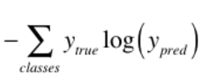
Pixel-wise loss function
The Pixel-wise Softmax with cross-entropy has nice differentiable properties, and therefore it is feasible for the optimization process.
But—
The same fails when you are dealing with a class imbalance.
Class imbalance can be defined as the examples which are well defined or annotated for training and examples which aren’t well-defined. A good example can be medical images or CT scans. CT scans are very dense in information and sometimes radiologists can fail to annotate anomalies properly.
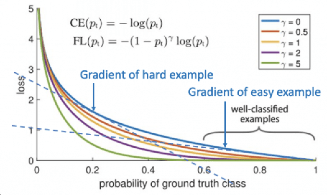
To intuitively understand the problem, let’s refer to the graph above.
The blue line indicates the highest loss throughout the graph. When the loss is higher the model receives unwanted signals, and learning is not optimum. That’s why we reduce the loss.
When it comes to imbalanced data, we want to quickly reduce the loss of the well-defined example. Simultaneously, when the model receives hard and ambiguous examples, the loss increases, and it can optimize that loss rather than optimizing loss on the easy examples.
The green line at the bottom of the graph shows the alternative methods that have been used to reduce the loss.
In order to tackle class imbalance by reducing easy loss, it’s recommended to employ Focal Loss.
Focal Loss
The Focal loss modifies the Pixel-wise Softmax with cross-entropy by quantitatively reducing the loss of the well-defined examples.
This is done by introducing a new term (1-pt ) where pt is the example and an exponential term gamma which controls and reduces the loss function. The exponential term gamma automatically reduces the contribution of easy examples at training time and focuses on the hard ones.
Essentially, the idea here is to reduce the effect of the easy examples on the model and ask it to focus on the more complex examples.

Focal loss function
Dice Loss
Another important function is the Dice function, which uses the dice coefficient to estimate the overlapping of the pixels of the predicted labels with the ground truth label.
The dice coefficient ranges from 0 to 1, where 1 denotes the perfect and complete overlap of pixels.
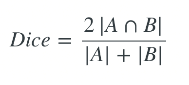
Dice loss function
Semantic Segmentation real-world applications
Semantic Segmentation has a lot of applications.
It has found its way to almost all the tasks related to images and video. Semantic Segmentation is used in image manipulation, 3D modeling, facial segmentation, the healthcare industry, precision agriculture, and more.
Pro tip: Check out 27+ Most Popular Computer Vision Applications and Use Cases.
Here are a few examples of the most common Semantic Segmentation use cases.
Self-driving cars
Self-driving cars require image capturing sensors that could enable them to visualize the environment, make decisions and navigate accordingly.
Semantic segmentation allows for an effective differentiation between various objects.
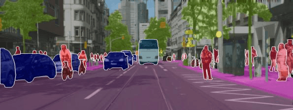
In the image above, you can see how the different objects are labeled using segmentation masks; this allows the car to take certain actions.
For instance, segmentation masks classifying pedestrians crossing the road will make the car stop, while segmentation classifying roads and lane marking will make the car follow a particular trajectory.
Medical image diagnosis
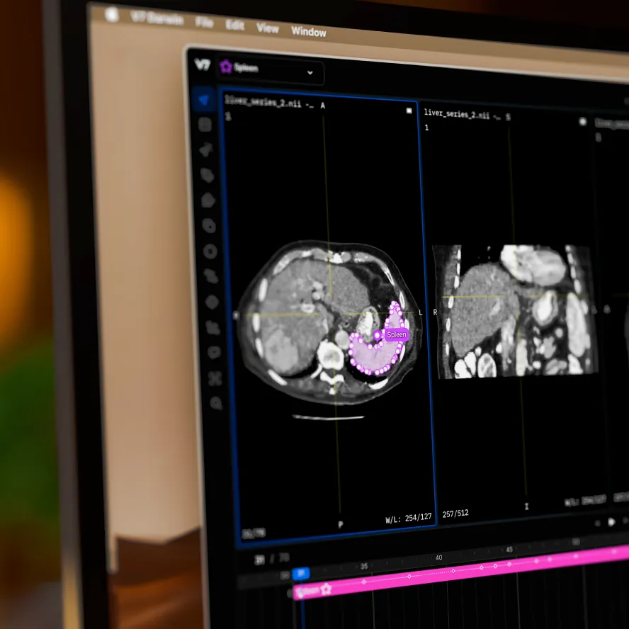
Semantic segmentation has also found its way in medical image diagnosis.
These days, radiologists find it very useful to classify anomalies in CT scans. CT scans and most medical images are very complex, which makes it hard to identify anomalies.
Semantic segmentation can offer itself as a diagnostic tool to analyze such images so that doctors and radiologists can make vital decisions for the patient’s treatment.
Here’s how you can perform medical image annotation using V7.
Pro tip: Are you looking for quality medical image data? Check out 21+ Best Healthcare Datasets for Computer Vision.
Scene understanding
Scene understanding applications require the ability to model the appearance of various objects in the scene like building, trees, roads, billboards, pedestrians, etc.
The model must learn and understand the spatial relationship between different objects.
For instance, in typical road scenes, the majority of the pixels belong to objects such as roads or buildings, and hence the network must yield smooth segmentation.

Aerial image processing
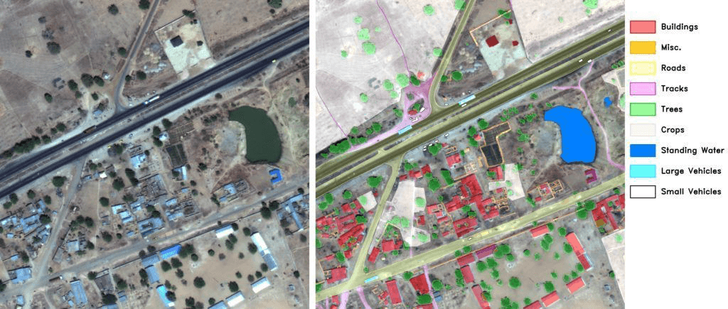
Aerial image processing is similar to scene understanding, but it involves semantic segmentation of the aerial view of the landscape.
This type of technology is very useful in times of crisis like a flood, where drones can spread to survey different areas to locate people and animals who need rescues.
Another area where aerial image processing can be used is the air delivery of goods.
Pro tip: See our list of 20+ Open Source Computer Vision Datasets to find quality image and video data for your projects.
Semantic Segmentation: Key Takeaways
Here’s a short recap of everything we’ve covered:
Semantic Segmentation is a technique that enables us to differentiate different objects in an image.
It can be considered an image classification task at a pixel level.
The deep learning methods we discussed for the task of semantic segmentation have fastened the development of algorithms that can be used in real-world scenarios with promising results.
These algorithms primarily use convolutional neural networks and their modified variants to get as accurate results as possible.
Loss functions allow us to optimize the neural network by reducing the error generated during the training process.
Semantic Segmentation finds applications in fields like autonomous driving, medical image analysis, aerial image processing, and more.
Read more:
Data Cleaning Checklist: How to Prepare Your Machine Learning Data
15+ Top Computer Vision Project Ideas for Beginners
YOLO: Real-Time Object Detection Explained
The Beginner’s Guide to Contrastive Learning
9 Reinforcement Learning Real-Life Applications
Mean Average Precision (mAP) Explained: Everything You Need to Know
Nilesh Barla is the founder of PerceptronAI, which aims to provide solutions in medical and material science through deep learning algorithms. He studied metallurgical and materials engineering at the National Institute of Technology Trichy, India, and enjoys researching new trends and algorithms in deep learning.
