Computer vision
Deep Learning for Image Super-Resolution [incl. Architectures]
17 min read
—
Jul 7, 2022
In this guide to image super-resolution, we discuss different evaluation techniques, learning strategies, architectures, as well as supervision methods.

Guest Author
The resolution of an image is the number of pixels displayed per square inch (PPI) of a digital image. Super-Resolution (SR) refers to enhancing the resolution of an image (or any type of signal like video sequences) from its low-resolution counterpart(s).
For example, when you zoom in on a digital image, you start seeing the image starting to get blurry. This is because the pixel density in the zoomed region is just linear interpolation which is not enough to portray a clear image.
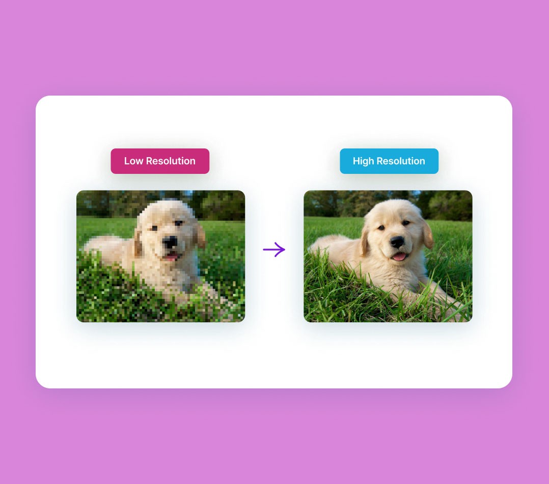
Here’s an example of SR aiming to obtain the HR image when given an LR image:
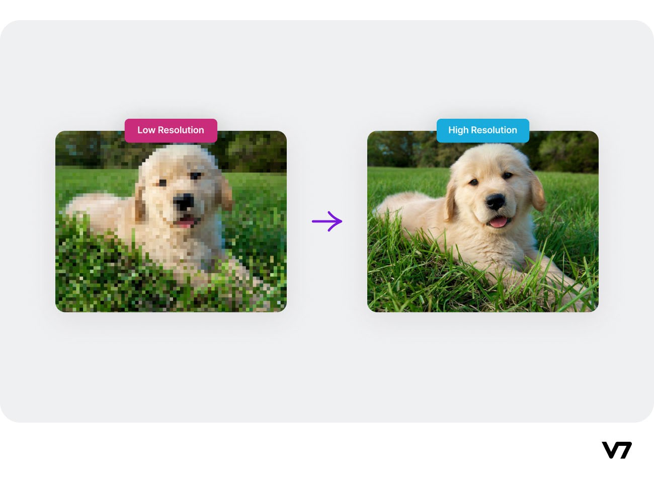
Low Resolution image (LR) and High Resolution image (HR) counterparts
Deep Learning techniques have been key to improving Super-Resolution technology due to their automatic feature extraction capabilities. Recent efforts have even focused on reducing the need for high-resolution images as ground truths for training neural networks.
In this article, we’ll cover:
Image Super-Resolution Essentials
Single-Image vs. Multi-Image Super-Resolution
Evaluation Techniques
Popular Architectures
Low Supervision Methods
Let’s dive in!
Image Super-Resolution Essentials
As mentioned earlier, Super-Resolution refers to increasing the resolution of an image. Suppose an image is of resolution (i.e., the image dimensions) 64x64 pixels and is super-resolved to a resolution of 256x256 pixels. In that case, the process is known as 4x upsampling since the spatial dimensions (height and width of the image) are upscaled four times.
Now, a Low Resolution (LR) image can be modeled from a High Resolution (HR) image, mathematically, using a degradation function, delta, and a noise component, eta as the following:

In supervised learning methods, models aim to purposefully degrade the image using the above equation and use this degraded image as inputs to the deep model and the original images as the HR ground truth. This forces the model to learn a mapping between a low-resolution image and its high-resolution counterpart, which can then be applied to super-resolve any new image during the testing time.
One question you might have is, “How good really is Super-Resolution?” Well, SR can yield extremely high-quality results in practical applications. For example, even though we can detect far away stars and planets, we can only capture blurry images of them even using large telescopes like the Hubble Space Telescope. Due to the advancements in SR techniques, we have been able to get clearer pictures of the celestial bodies.
The first-ever image of the black hole, which is located millions of light-years away from us, was not technically “captured.” The information captured was super-resolved to the final image we have now. SR technology has far passed its infant stage and is now being applied to areas like military, surveillance, biomedical imaging (especially in microscopic studies), etc. The recent focus of SR research is on reducing the need for labeled samples since we have already attained peak results using Supervised Learning.
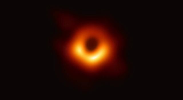
First ever image of the black hole. Source: JPL, Caltech
Single-Image vs. Multi-Image Super-Resolution
Two types of Image SR methods exist depending on the amount of input information available. In Single-Image SR, only one LR image is available, which needs to be mapped to its high-resolution counterpart. In Multi-Image SR, however, multiple LR images of the same scene or object are available, which are all used to map to a single HR image.
In Single-Image SR methods, since the amount of input information available is low, fake patterns may emerge in the reconstructed HR image, which has no discernible link to the context of the original image. This can create ambiguity which in turn can lead to the misguidance of the final decision-makers (scientists or doctors), especially in delicate application areas like bioimaging.
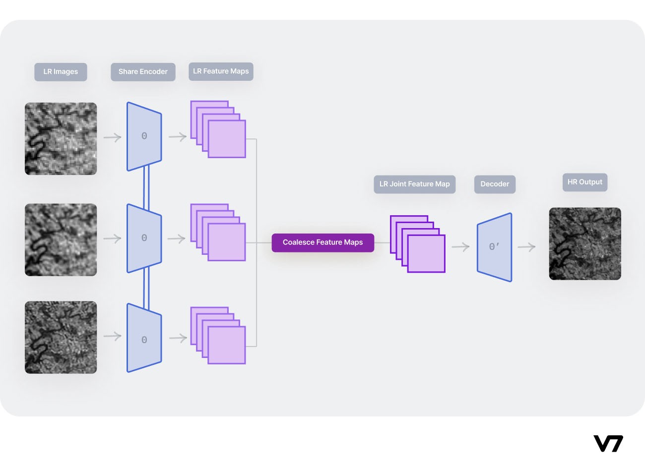
Typical workflow of Multi-Image Super-Resolution Methods. Image by the author.
Intuitively, we can conclude that Multi-Image SR produces better performance since it has more information to work with. However, the computational cost in such cases is also increased several-fold, making it infeasible in many application scenarios where there is a substantial resource constraint. Also, obtaining multiple LR images of the same object is tedious and not practical. Thus, Single-Image SR is more closely related to the real world, although it is a more challenging problem statement.
In fully supervised Multi-Image SR methods, typically, different degradation functions are used on the HR image (the ground truths) to obtain slightly different types of LR images for the same scene. This helps the model make better generalizations thanks to the diversity of available information. In other cases, augmented versions (rotation, flipping, affine transform, etc.) of the same LR image are used.
One example of a simple Multi-Image SR model is the MISR-GRU model proposed in this paper, where each of the available LR images was separately embedded in feature space using the same encoding network. Then these multiple feature maps were fused using the Convolutional Gated Recurrent Unit (ConvGRU) model (which is a Recurrent Neural Network). Finally, the fused feature map was passed through deconvolution layers to reconstruct the HR image. The architectural overview of their method is shown below:

Source: Paper
Evaluation Techniques
Visual cues are not enough to evaluate and compare the performance of different SR methods since they are very subjective in nature. A universal quantitative measure of SR performance is required to compare models in a fair way.
Peak Signal-to-Noise Ratio (PSNR) and Structural SIMilarity (SSIM) Index are the two most commonly used evaluation metrics for evaluating SR performance. PSNR and SSIM measures are generally both used together for a fair evaluation of methods compared to the state-of-the-art.
Let us discuss these metrics next.
PSNR
Peak Signal-to-Noise Ratio or PSNR is an objective metric that measures the quality of image reconstruction of a lossy transformation. Mathematically it is defined by the following:

Here, “MSE” represents the pixel-wise Mean Squared Error between the images, and “M” is the maximum possible value of a pixel in an image (for 8-bit RGB images, we are used to M=255). The higher the value of PSNR (in decibels/dB), the better the reconstruction quality.
SSIM
The Structural SIMilarity (SSIM) Index is a subjective measure that determines the structural coherence between two images (the LR and super-resolved HR images in this case). Mathematically it can be defined as follows:


SSIM ranges between 0 and 1, where a higher value indicates greater structural coherence and thus better SR capability.
Learning Strategies
Image SR models use different strategies for super-resolving images- typically, the key difference lies in the upsampling technique for obtaining the final HR output. Let us discuss these techniques next and see the relative benefits and demerits.
Pre Upsampling
In this class of methods, the LR input image is first upsampled to meet the dimensions of the required HR output. Then processing is done on the upscaled LR image using a Deep Learning model.
VDSR is an early attempt at the SR problem that uses the Pre Upsampling method. The VDSR network utilizes a very deep (20 weight layers) convolutional network (hence the name) inspired by VGG networks.
Pro Tip: Read this Comprehensive Guide to Convolutional Neural Networks
Typically deep networks converge slowly if the learning rates are low. However, boosting convergence and high learning rates might lead to exploding gradients. Thus, in VDSR, residual learning and gradient clipping has been used to address these issues. Further, VDSR tackles multi-scaled SR problems using just one network. VDSR’s network architecture is shown below.
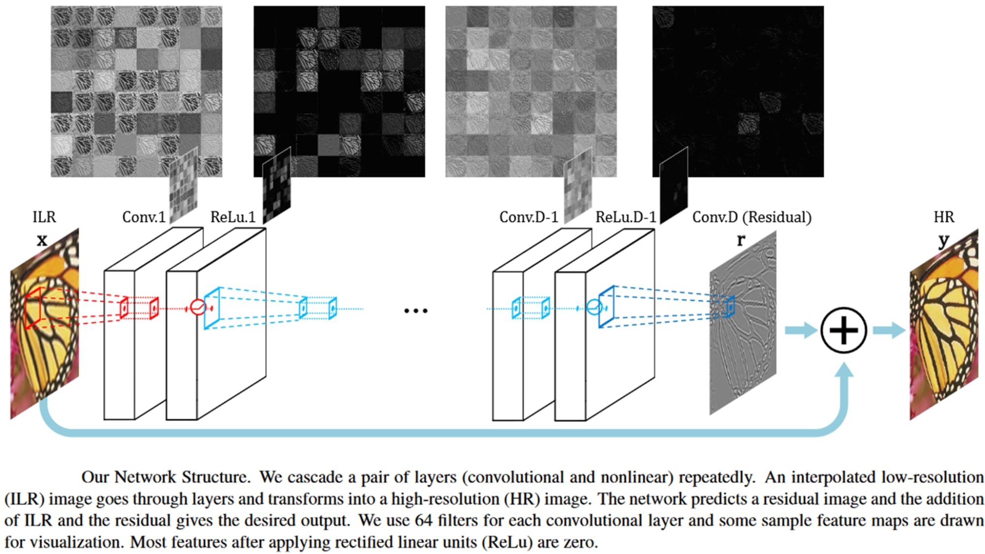
Source: Paper
An example of a super-resolved image obtained by the VDSR network compared to the then state-of-the-art is shown below.
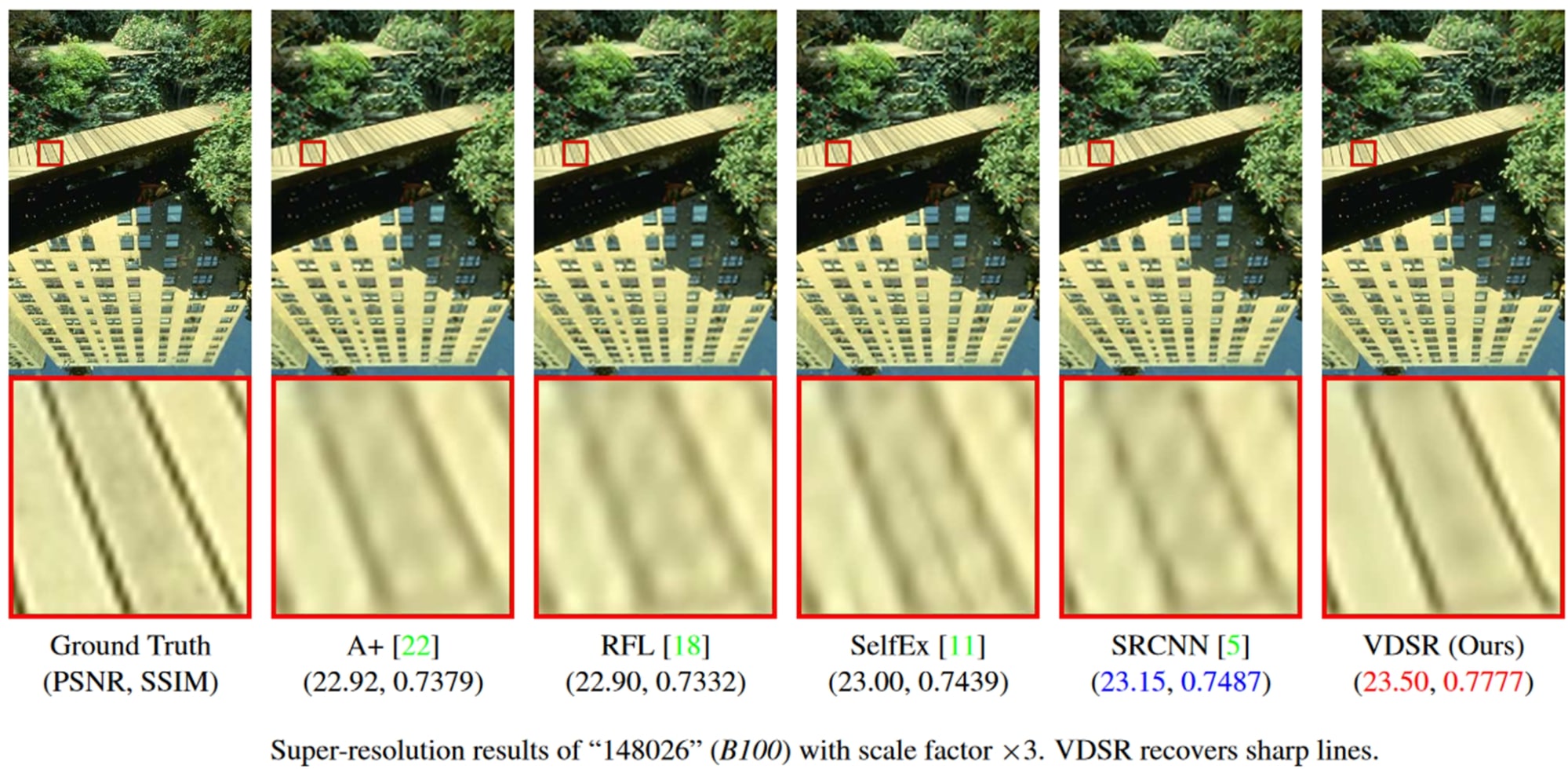
Source: Paper
Post Upsampling
Increasing the resolution of the LR images (in Pre Upsampling methods) before the image enhancement step increases the computational complexity. This is especially problematic for convolutional networks, where the processing speed directly depends on the input image resolution. Secondly, interpolation methods typically used to accomplish the task, such as bicubic interpolation, do not bring additional information to solve the ill-posed reconstruction problem.
Thus, in the Post Upsampling class of SR methods, the LR image is first processed for enhancement using a deep model, and then it is upscaled using traditional techniques like bicubic interpolation to meet the HR image dimension criteria.
FSRCNN is a popular SR model (an improvement to the SRCNN model) that uses the Post Upsampling technique. In the FSRCNN architecture, the feature extraction is performed in the LR space. FSRCNN also uses a 1x1 convolution layer after feature extraction to reduce the computational cost by reducing the number of channels. The architecture of the FSRCNN model is shown below.
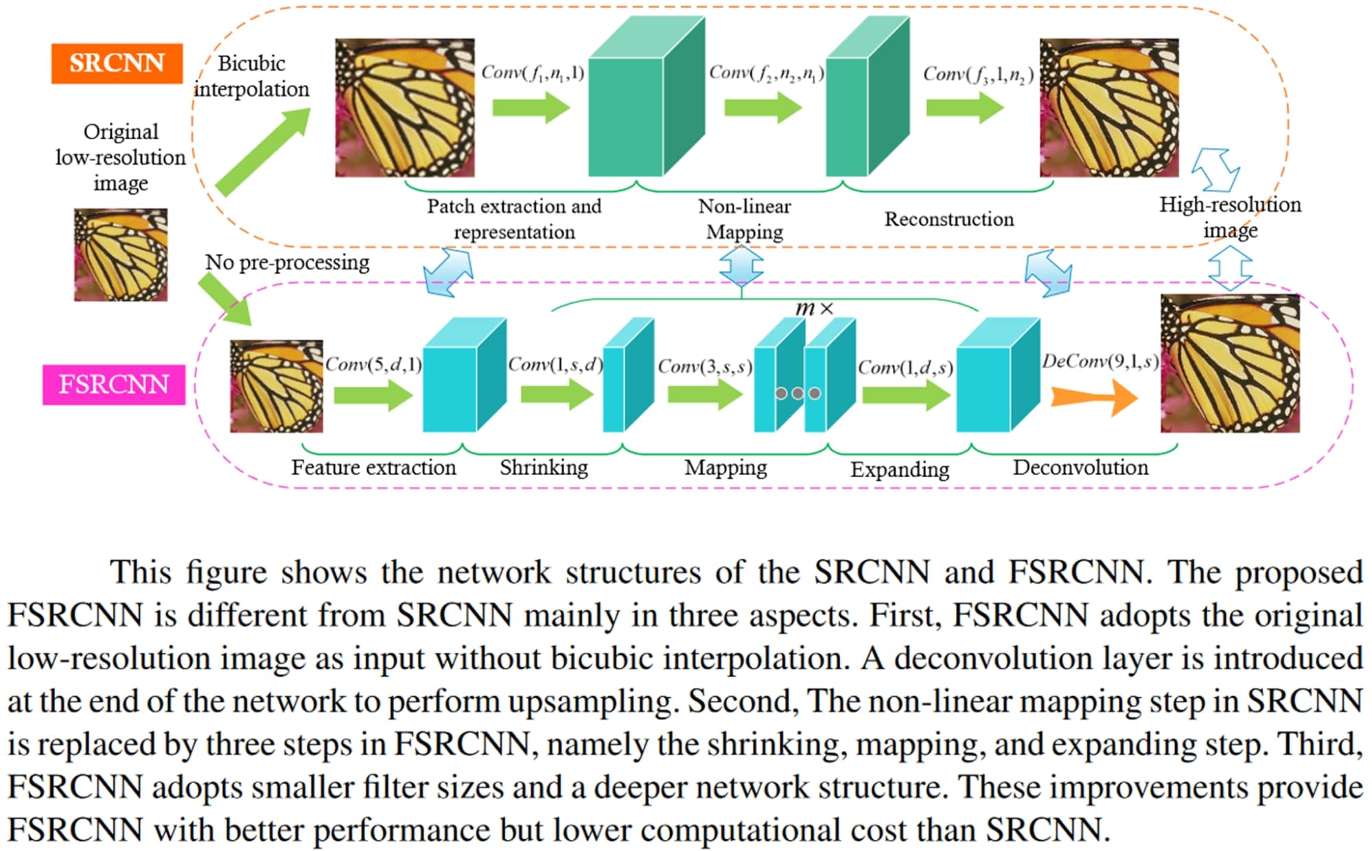
Network structures of the SRCNN and FSRCN. Source: Paper
Some results obtained by the FSRCNN model when compared to the state-of-the-art methods are shown below. FSRCNN performed better than SRCNN while having a much lesser computational cost.
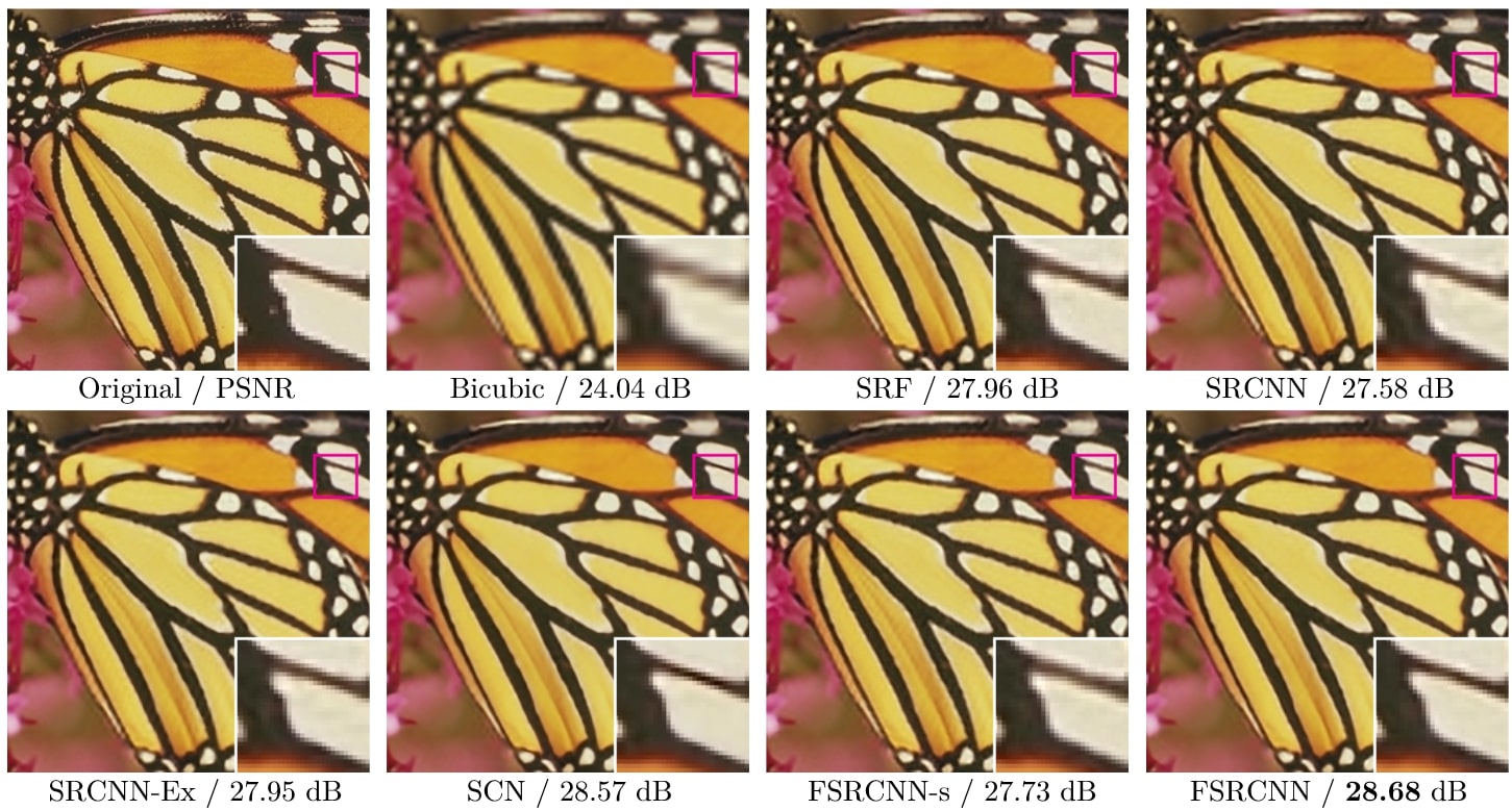
Source: Paper
Progressive Upsampling
Pre and Post Upsampling methods are both useful methods. However, for problems where LR images need to be upscaled by large factors (say 8x), regardless of whether the upsampling is done before or after passing through the deep SR network, the results are bound to be suboptimal. In such cases, it makes more sense to progressively upscale the LR image to finally meet the spatial dimension criteria of the HR output rather than upscaling by 8x in one shot. Methods that use this strategy of learning are called Progressive Upsampling methods.
One such model is the LapSRN or Laplacian Pyramid Super-Resolution Network architecture which progressively reconstructs the sub-band residuals of HR images. Sub-band residuals refer to the differences between the upsampled image and the ground truth HR image at the respective level of the network. The network architecture of LapSRN juxtaposed to other traditional architectures is shown below.
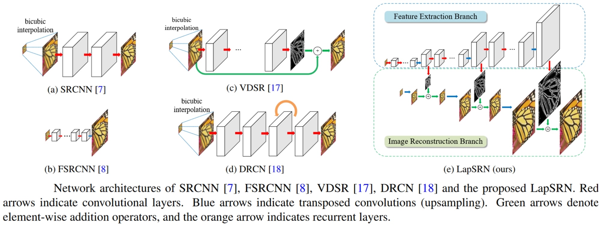
Source: Paper
LapSRN is based on a cascade of CNNs. LapSRN takes an LR image as input and progressively predicts the sub-band residuals in a coarse-to-fine fashion. At each level, LapSRN first applies a cascade of convolutional layers to extract varied feature maps. Then a transposed convolutional layer is used for upsampling the feature maps to a finer level. Finally, a convolutional layer is employed to predict the sub-band residuals. The predicted residuals at each level are used to efficiently reconstruct the HR image through upsampling and addition operations. LapSRN generates multiple intermediate SR predictions in one feed-forward pass through progressive reconstruction using the Laplacian pyramid.
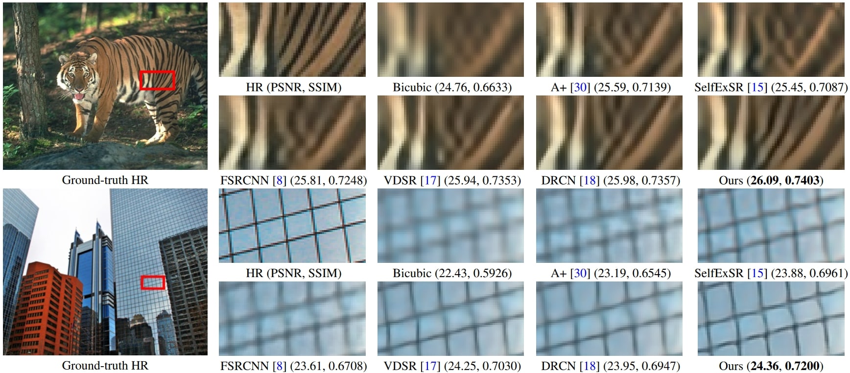
Examples of results obtained by the LapSRN model compared to the state-of-the-art methods are shown below.
Source: Paper
Popular Architectures
Several Deep Learning-based models have been proposed over the years to address the SR problem, some of which were revolutionary at the time, becoming the stepping stones for future research in SR technology. Let us discuss some of the most popular SR architectures next.
SRCNN
One of the earliest approaches to the SR problem using Deep Learning includes the SRCNN (Super-Resolution Convolutional Neural Network) model proposed in this paper in 2015. SRCNN is a fully convolutional network, and the primary focus of the model was the simplicity of the architecture and fast processing speeds.

Source: Paper
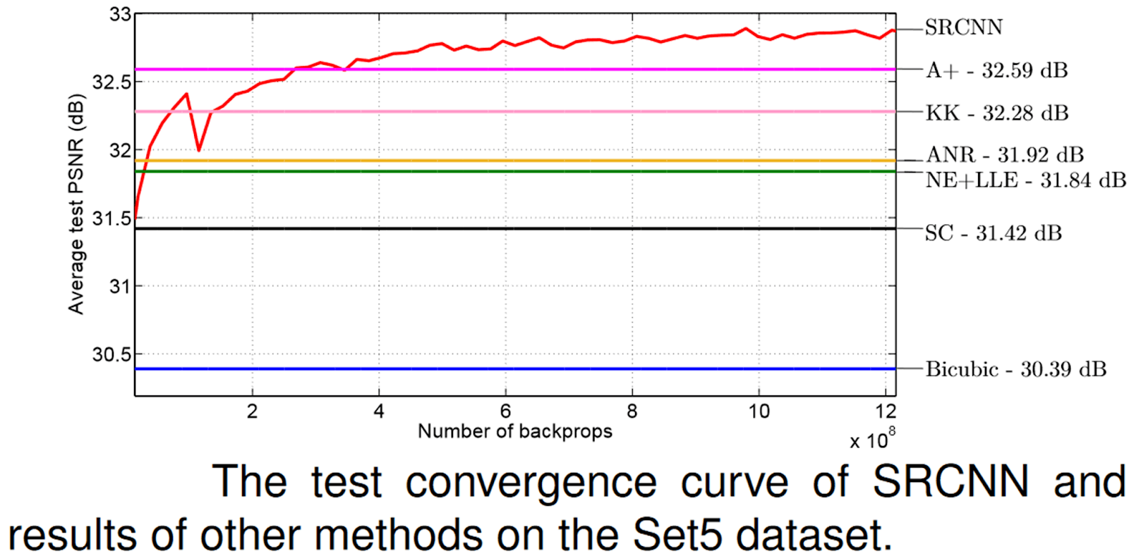
An overview of the SRCNN model is shown above. SRCNN produced better results with lesser computational costs as compared to the traditional SR methods that were popular at the time. A comparison of the results (both qualitative and quantitative) is shown below, where SRCNN was compared with Bicubic Interpolation and Sparse-Coding (SC) methods and some other state-of-the-art models at the time.

Source: Paper
Source: Paper
SRGAN
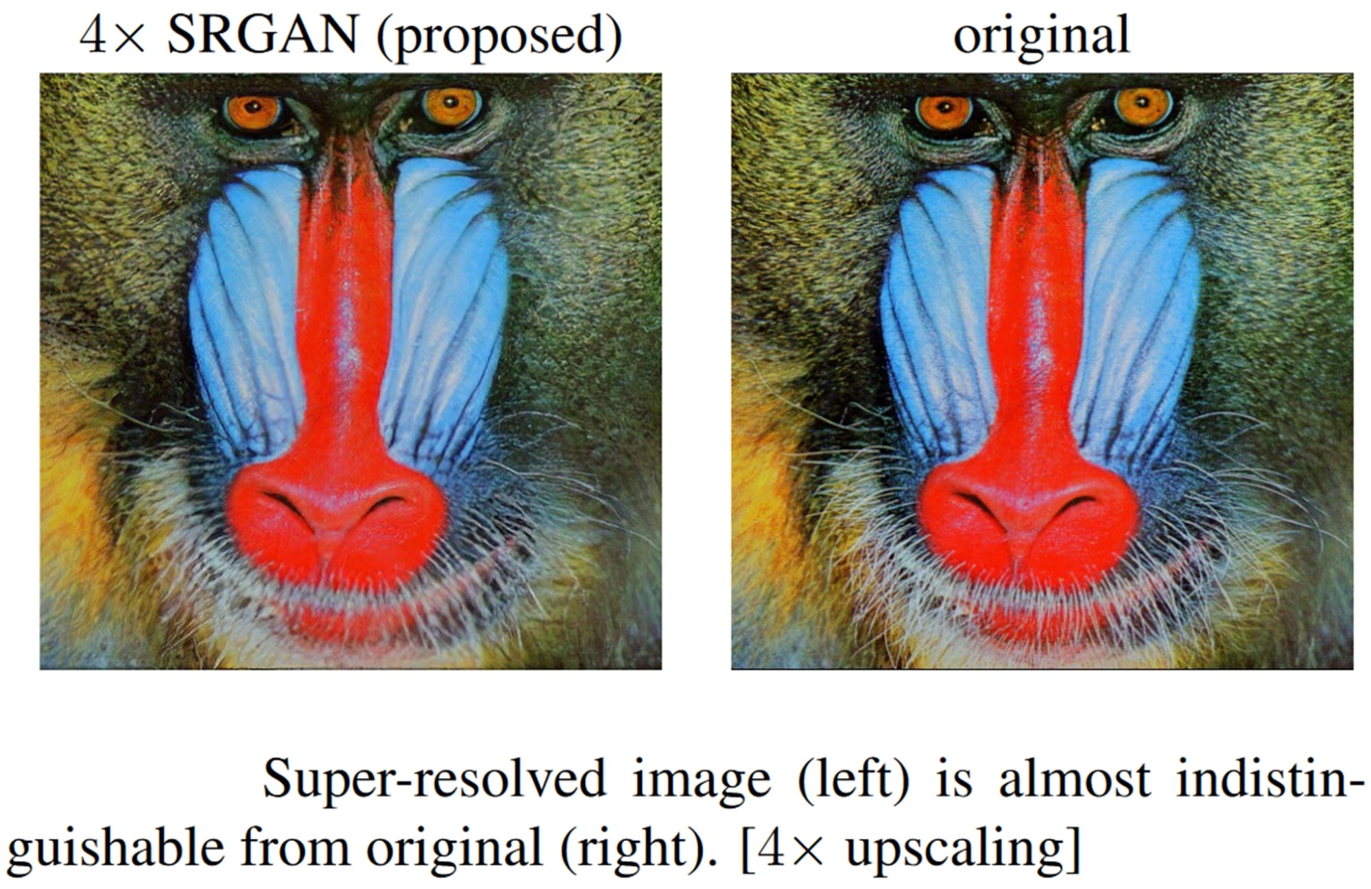
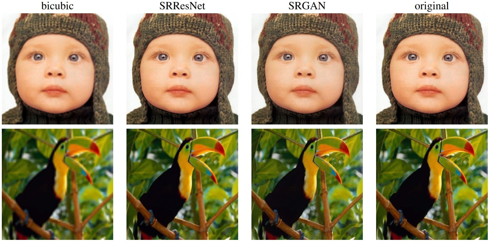
The SRGAN model, proposed in this paper, was a revolutionary model in the SR literature since it was the first method that could super-resolve photo-realistic natural images at 4x upsampling (an example of which is shown below).
Source: Paper
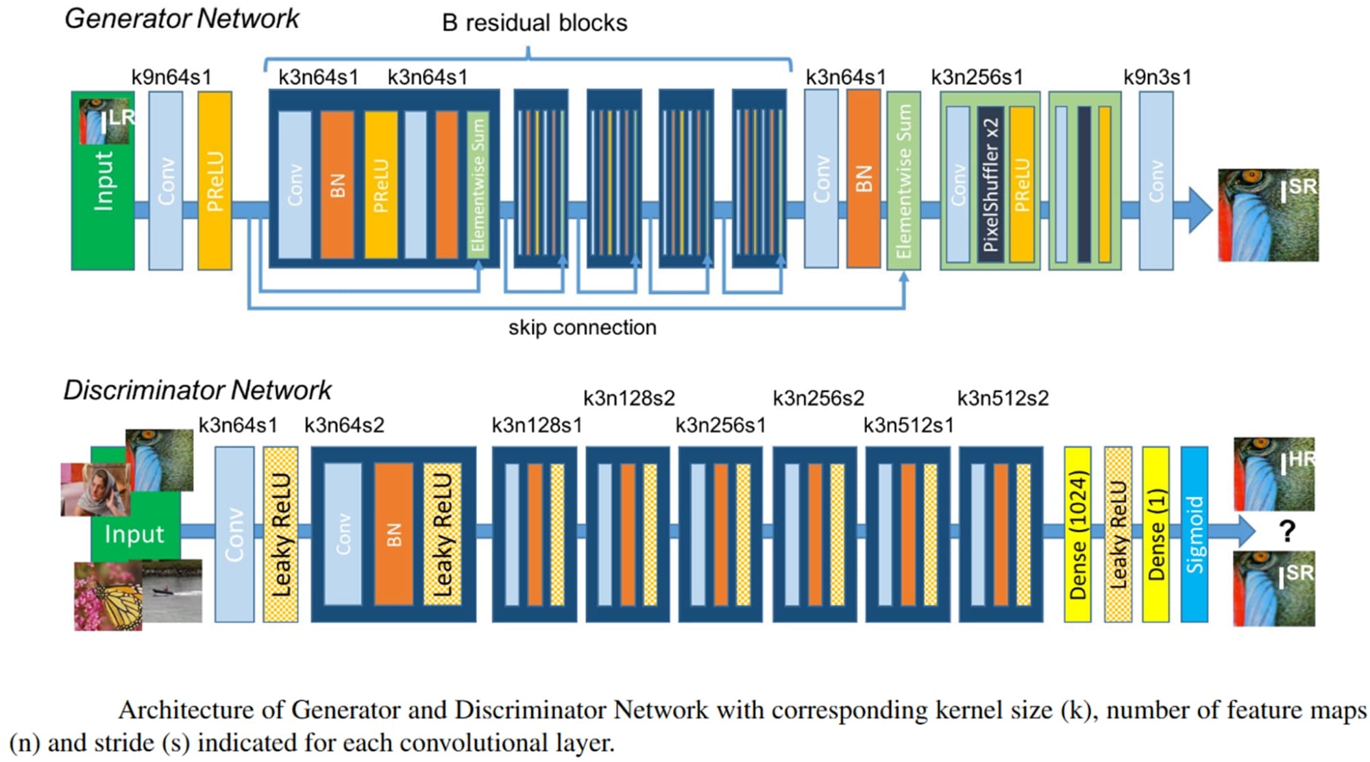
SRGAN is a Generative Adversarial Network-based (GAN) model that employs a deep (16 blocks) residual network with skip connections. While most SR approaches had used minimization of the Mean-Squared Error (MSE) as the only optimization target, SRGAN is optimized for a new perceptual loss, enabling SRGAN to produce super-resolved images with high upscaling factors. SRGAN calculates the loss on the feature maps of a VGG Network instead of the traditional MSE loss. The architecture of SRGAN is shown below.
Source: Paper
Some visual results obtained by the SRGAN model compared to other methods are shown below.
Source: Paper
ESPCN
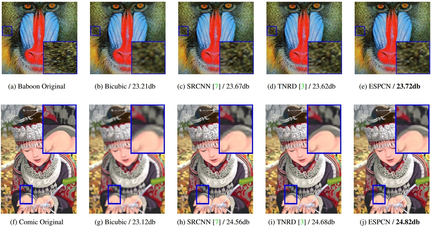
ESPCN is a Post Upsampling method of SR, where upscaling is handled by the last layer of the network, and super-resolution of the LR input to the HR image is accomplished from LR feature maps. To do this, the authors proposed an efficient sub-pixel convolution layer to learn the upscaling operation for image SR. This means that a convolution operation with a fractional stride is performed in the LR space. This activates different parts of the convolution filters depending on the location of the sub-pixels, which saves a lot of computational costs. The architecture of the ESPCN model is shown below.

Source: Paper
Some results obtained by the ESPCN model compared to the then state-of-the-art models (which use Pre Upsampling techniques) are shown below.
Source: Paper
SwinIR
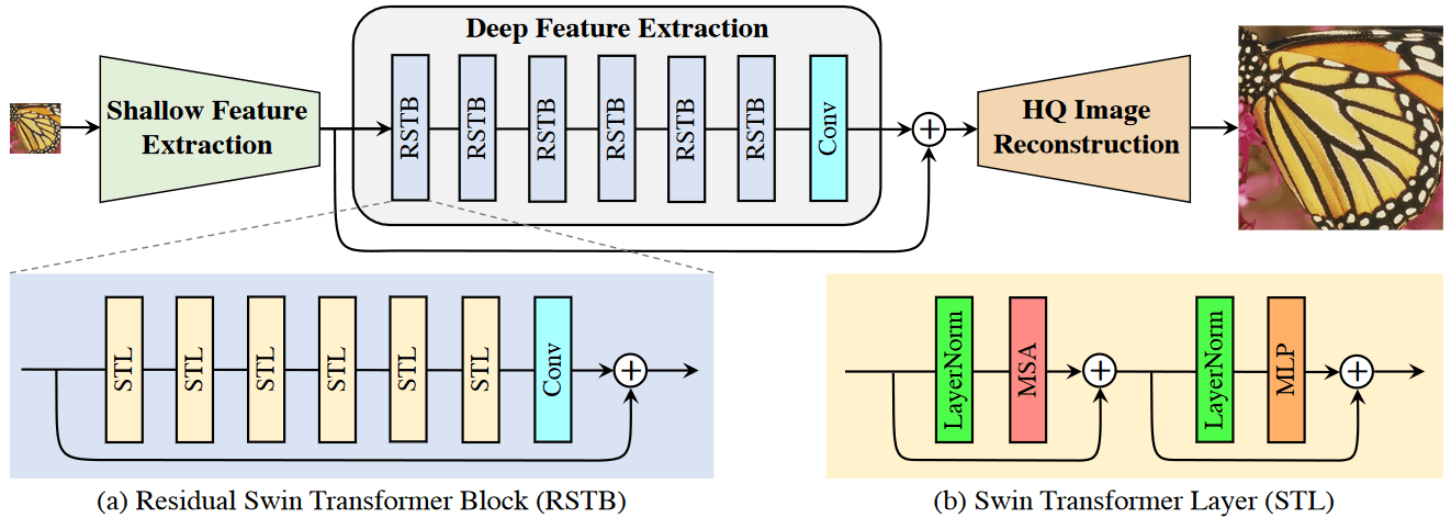
SwinIR is a recently proposed image reconstruction method that utilizes the widely popular Swin Transformer network, which integrates the advantages of both CNNs and Transformers. SwinIR consists of three modules: shallow feature extraction, which uses a single convolution layer that is directly transmitted to the reconstruction module to preserve low-frequency information; a deep feature extraction module which is mainly composed of residual Swin Transformer blocks, each of which utilizes several Swin Transformer layers for local attention and cross-window interaction; and finally, high-quality image reconstruction modules where both shallow and deep features are fused. The architecture of the SwinIR model is shown below.
Source: Paper
An example of visual results obtained by the SwinIR model compared to popular SR methods is shown below, which clearly showcases SwinIR’s superiority.

Source: Paper. (Best viewed when zoomed)
The most distinguishing feature about SwinIR is that it achieves state-of-the-art results while having up to 67% fewer parameters than most previous SR models.

Source: Paper
Low Supervision Methods
Most of the popular methods in SR use fully supervised learning to train large networks. However, such methods work reliably only when there is a large quantity of high-quality ground truth labels. Such large amounts of labeled data are challenging to obtain because data labeling is a time-consuming and costly operation. 80% of the total time spent on a supervised Machine Learning project goes towards data curating. Moreover, in medical SR tasks, it becomes costly since only expert doctors can annotate the data.
Thus, reducing the requirement of labeled data for solving the SR problem has been the focus of researchers in the last few years. Although not always as good as supervised learning, such low supervision methods yield excellent results. Let us discuss some of the low-supervision techniques in SR.
Semi-Supervised Methods
Semi-Supervised Learning is a paradigm where, in a large dataset, only a small percentage of the data is labeled. That is, deep models have access to a large amount of unstructured data, along with a small set of labeled data for network training.
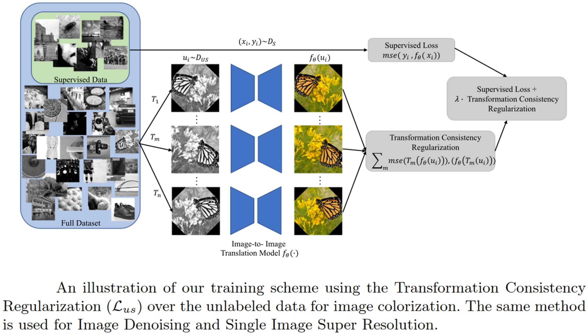
One such approach was taken in this paper, where the authors used only 10-20% labeled data. The authors, taking insights from the Consistency Regularization literature, introduce a regularization term over the unsupervised data called Transformation Consistency Regularization (TCR), which makes sure the model’s prediction for a geometric transform of an image sample is consistent with the geometric transformation of the model’s reconstruction of the image.
If we rotate an image by 45 degrees and super-resolve it, the obtained output should be identical to an output obtained by first super-resolving the original image and then rotating it by 45 degrees. Their training scheme is shown below.
Source: Paper
Few-Shot Methods
Few-Shot Learning is a meta-learning mechanism (meta-learning means learning to learn) where a pre-trained model is extended to new data patterns by using only a handful of labeled samples. This paper introduced Few-Shot Learning in the SR problem for the first time, where they used graphical modeling.
The authors introduced a Distortion Relation Network (DRN) to learn the expected distortion-relation embeddings. To make the DRN general for arbitrary image SR, they designed a prior knowledge memory bank to store the learnable distortion-relation from seen auxiliary tasks (i.e., synthetic distortions using degradation functions). Thus, given an arbitrary real distorted sample, it can traverse the prior knowledge memory bank to acquire the needed distortion embeddings.
Then similarities between the distortions are drawn using cosine similarity, and a “Distortion-Relation guided Transfer Learning” (DRTL) network proposed by the authors is used for obtaining the final super-resolved output. The diagram of the DRN is shown below.

Source: Paper
Some visual results obtained by the DRN and other baseline results are shown below.
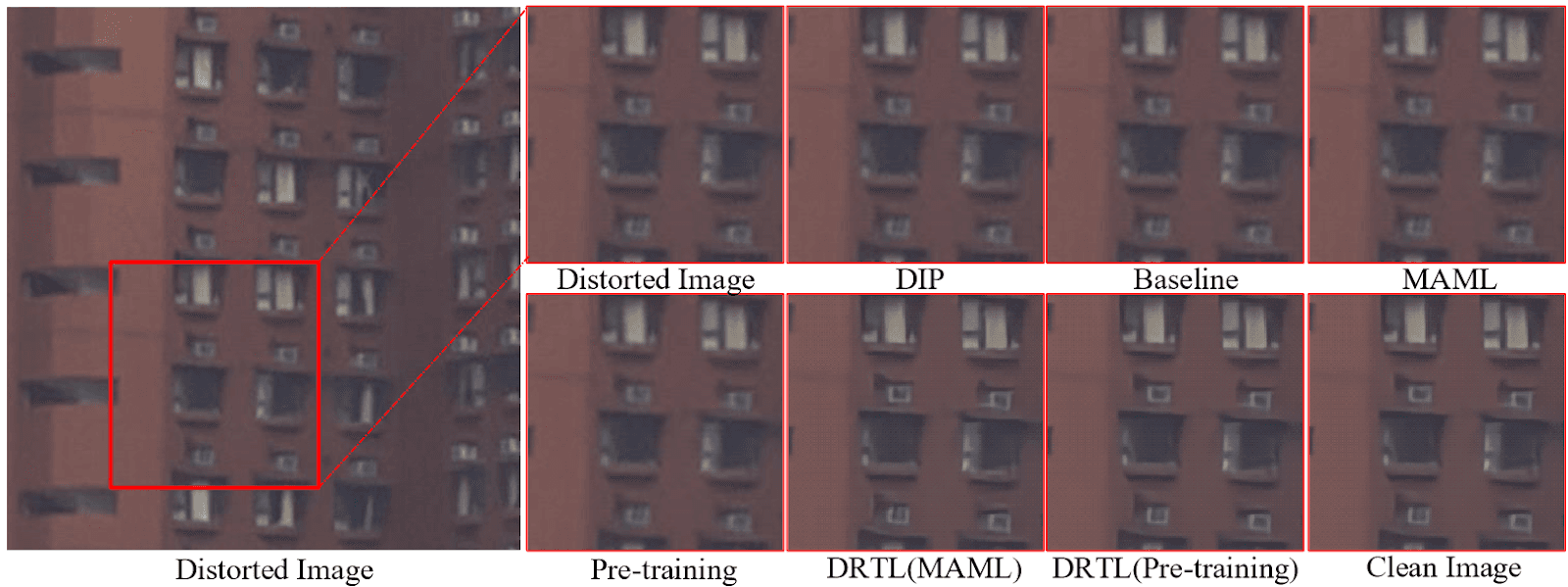
Source: Paper. (Best viewed when zoomed)
Unsupervised Methods
Unsupervised Learning is a Machine Learning paradigm where all the data available for training a deep model is unstructured, i.e., ground truths are entirely missing. This makes the SR problem even more challenging.
One method that tackles such a problem setting is the CinCGAN model, which utilizes a Cycle-in-Cycle structure inspired by the popular CycleGAN model (which was proposed for general-purpose image-to-image translation). In CycleGAN, the dimensions of the input and output images are the same, which is not the case in SR problems.
CinCGAN consists of two CycleGANs where the first CycleGAN maps the LR input image to the clean and bicubic downsampled LR space. Then a pre-trained deep model with bicubic downsampling assumption is stacked on top of it to up-sample the intermediate result to the desired size. The entire first CycleGAN model acts as one of the generators of the second CycleGAN model. Adversarial Learning is used to fine-tune the entire network. The architecture diagram for CinCGAN is shown below.

Source: Paper
The yellow dotted lines above show the first CycleGAN module, which acts as a generator for the second CycleGAN model. Some results obtained by the CinCGAN model are shown below. The unsupervised approach yields results that are, on occasions, even better than fully supervised approaches (like the EDSR model in the comparison).
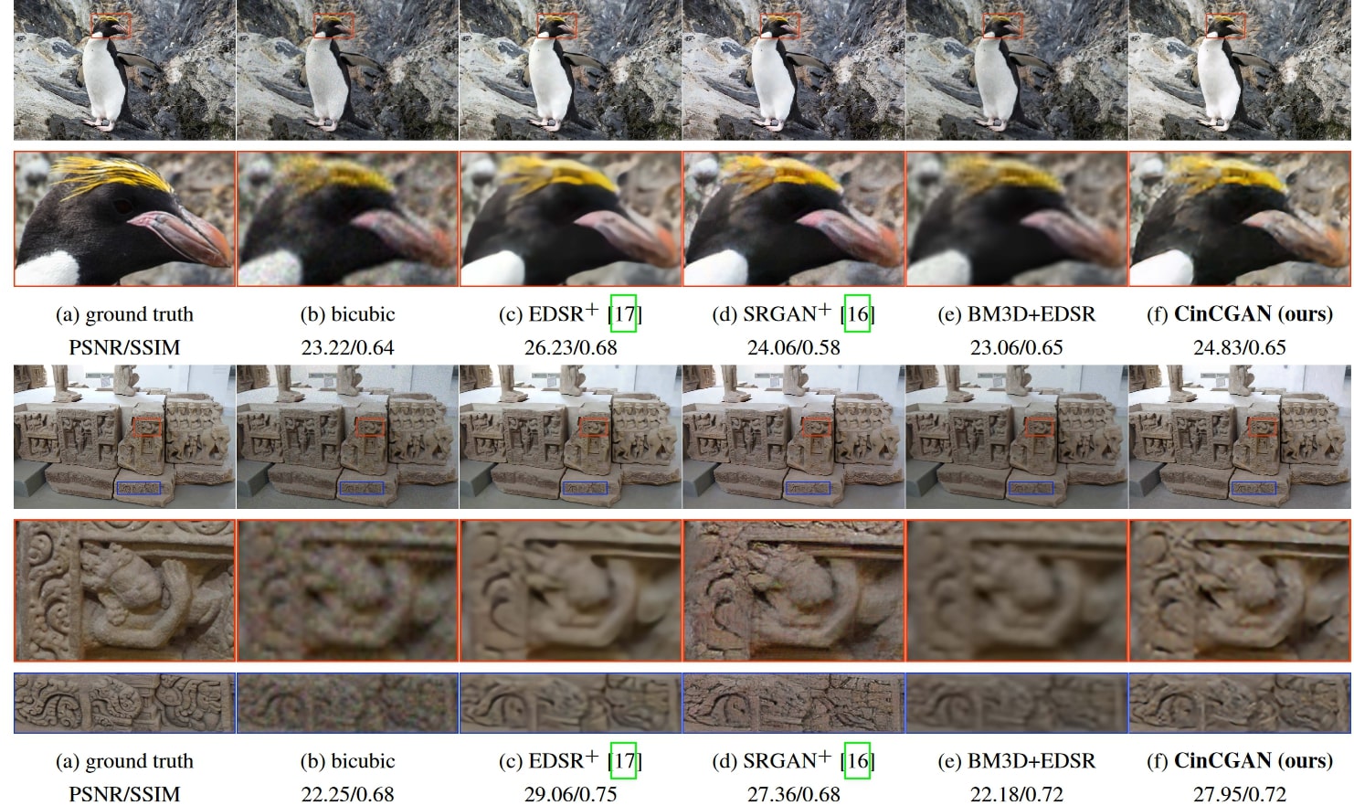
Source: Paper
Self-Supervised Methods
Self-Supervised Learning is essentially a subset of Unsupervised Learning since this too does not use any labeled data for drawing inference. However, in Self-Supervised Learning, the model generates labels for the unlabeled input data and, in future iterations, uses the generated labels to further refine the predictions. This cumulative, iterative process continues till an end criterion is reached.
One example of a method that utilizes Self-Supervised Learning for SR is the High Dynamic Range Deep Shift-and-Pool or HDR-DSP model proposed in this paper for multi-image SR. In multi-image SR for Self-Supervised Learning, instead of using ground truth labels, one of the degraded frames in the input sequence is withheld from the network and used as a label.
HDR-DSP is able to handle a variable number of input frames and is robust to errors in the exposure times. A shift-and-pool module merges the feature maps obtained from each LR image into an HR feature map by temporal pooling using permutation invariant statistics: the maximum and standard deviation of pixel values. The architecture of the HDR-DSP model is shown below.

Source: Paper
Some results obtained by the authors are shown below. The results obtained by the HDR-DSP model, when compared to previous state-of-the-art methods, show its superiority, considering that no labeled samples were present for model training.

Source: Paper
Conclusion
Image Super-Resolution, which aims to enhance the resolution of a degraded/noisy image, is an important Computer Vision task due to its enormous applications in medicine, astronomy, and security. Deep Learning has largely aided in the development of SR technology to its current glory.
Multi-Image and Single-Image SR are the two distinct categories of SR methods. Multi-Image SR is computationally expensive but produces better results than Single-Image SR, where only one LR image is available for mapping to the HR image. In most applications, Single-Image SR resembles real-world scenarios more closely. However, in some applications, like satellite imaging, multiple frames for the same scene (often at different exposures) are readily available, and thus Multi-Image SR is used extensively.
While we have already achieved excellent results with SR technology, most of it has been achieved using fully Supervised Learning- which entails training a deep model with an enormous amount of labeled data. Such large quantities of data might not be readily available, especially in applications like medical imaging, where only expert doctors can annotate the data. Thus, recent SR research has focused on reducing or even eliminating any supervision from SR tasks.
