Blog

Webinar

Academy

Resources

Computer vision

Cross Entropy Loss: Intro, Applications, Code

12 min read

—

Jan 26, 2023

Let's dive into cross-entropy functions and discuss their applications in machine learning, particularly for classification issues.

Deval Shah

In 2023, machine learning is present in almost all applications we interact with daily.

To ensure the applications operate at maximum efficiency, all businesses must continuously optimize their ML models. Fine-tuning all parameters is the only way to create models that achieve the highest performance—and contribute to creating the best user experience.

One of these parameters is accuracy, measured with the loss function. And the most widely used loss function in machine learning applications is cross entropy.

In this article, we'll explain cross-entropy functions in detail and discuss their applications in machine learning, particularly for classification issues.

Here’s what we’ll cover:

What is cross entropy?
Loss functions in machine learning
Cross-entropy loss functions
How to apply cross entropy?

Data labeling

Data labeling platform

Get started today

Data labeling

Data labeling platform

Get started today

What is cross entropy?

Before delving into the concept of entropy, let’s explain the concept of information theory. It was first introduced by Claude Shannon in his groundbreaking work, 'A theory of communication,' in 1948.

According to Shannon, entropy is the average number of bits required to represent or transmit an event drawn from the probability distribution for the random variable.

In simple terms, entropy indicates the amount of uncertainty of an event. Let’s take the problem of determining the fair coin toss outcome as an example.

For a fair coin, we have two outcomes. Both have P[X=H] = P[X=T] = 1/2. Using the Shannon entropy equation:

Both terms are 0 for the coin, almost always H or almost always T, so the entropy is 0.

In the data science domain, the cross entropy between two discrete probability distributions is related to Kullback-Leibler (KL)Divergence, a metric that captures how similar the two distributions are.

Given a true distribution t and a predicted distribution p, the cross entropy between them is given by the following equation:

Cross entropy formula

Here, t and p are distributed on the same support S but could take different values.

For a three-element support S, if t = [t1, t2, t3] and p = [p1, p2, p3], it’s not necessary that t_i = p_i for i in {1,2,3}.

In the real world, however, the predicted value differs from the actual value, referred to as divergence, because it differs or diverges from the actual value. As a result, cross-entropy is the sum of Entropy and KL divergence (type of divergence).

Now let’s understand how cross-entropy fits in the deep neural network paradigm using a classification example.

Every classification case has a known class label, which has a probability of 1.0, whereas every other label has a probability of 0. Here, the model determines the probability that a particular case falls within each class name. Cross-entropy can then be used to determine how the neural pathways differ for each label.

Each predicted class probability is compared to the desired output of 0 or 1. The calculated score/loss penalizes the probability based on how far it is from the expected value. The penalty is logarithmic, yielding a large score for significant differences close to 1 and a small score for minor differences close to 0.

Cross-entropy loss is used when adjusting model weights during training. The aim is to minimize the loss—the smaller the loss, the better the model.

Cross entropy (classification) (source)

Loss functions in machine learning

A loss function measures how far the model deviates from the correct prediction.

Loss functions provide more than just a static illustration of how well your model functions; they also serve as the basis for how accurately your algorithms match the data. Most machine learning algorithms employ a loss function during the optimization phase, which involves choosing data's optimal parameters (weights).

Consider linear regression. Traditional "least squares" regression uses mean squared error (MSE) to estimate the line of best fit, hence the name "least squares"! The MSE is produced for weights the model tries across all input samples. Using an optimizer method like Gradient Descent, the model then reduces the MSE functions to the absolute minimum.

Machine learning algorithms usually have three types of loss functions.

Regression loss functions deal with continuous values, which can take any value between two limits., such as when predicting a country's GDP per capita, given its population growth rate, urbanization, historical GDP trends, etc.

Classification loss functions deal with discrete values, like classifying an object with a confidence value. For instance, image classification into two labels: cat and dog.

‍Ranking loss functions predict the relative distances between values. An example would be face verification, where we want to know which face images belong to a particular face. We can do so by ranking faces that do not belong to the original face-holder via their degree of relative approximation to the target face scan.

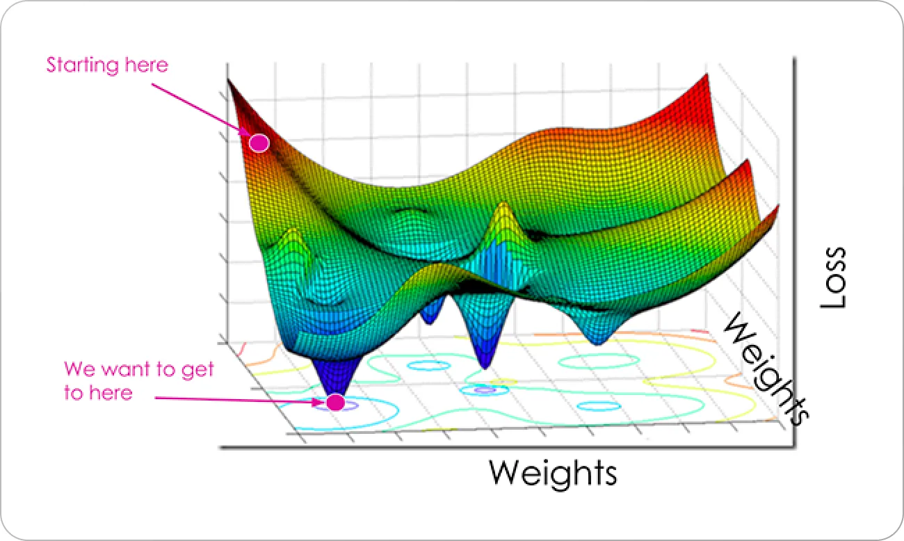
Loss landscape during model optimization (source)

Before we jump into the loss functions, let’s discuss activation functions and their applications. Output activation functions are transformations we apply to vectors coming out from Convolutional Neural Networks (CNNs) before the loss computations.

Sigmoid and Softmax have widely used activation functions in classification problems.

Read this detailed piece on PyTorch Loss Functions and start training your ML models.

Sigmoid

Sigmoid squashes a vector in the range (0, 1). It is applied independently to each input element in the batch during training. It’s also called the logistic function.

Sigmod function graph (source)

Softmax

Softmax is a function, not a loss. It squashes a vector in the range (0, 1), and all the resulting elements add up to 1. It is applied to the output scores s.

As elements represent a class, they can be interpreted as class probabilities. The Softmax function cannot be applied independently to each element si since it depends on all elements of s. For a given class si, the Softmax function can be computed as:

Softmax function (source)

Activation functions transform vectors before computing the loss in the training phase. In testing, activation functions are also used to get the CNN outputs when the loss is no longer applied.

Cross-entropy loss functions

Cross entropy extends the concept of information theory entropy by measuring the variation between two probability distributions for a given random variable/set of occurrences.

Cross-entropy loss is used when adjusting model weights during training. The aim is to minimize the loss—the smaller the loss, the better the model. A perfect model has a cross-entropy loss of 0. It typically serves multi-class and multi-label classifications.

Cross-entropy loss measures the difference between a deep learning classification model's discovered and predicted probability distributions.

The cross-entropy between two probability distributions, such as Q from P, can be stated formally as

H(P, Q)

Where:

H() is the cross-entropy function
P may be the target distribution
Q is the approximation of the target distribution.

Cross-entropy can be calculated using the probabilities of the events from P and Q:

H(P, Q) = — sum x in X P(x) * log(Q(x))

Usually, an activation function (Sigmoid/Softmax) is applied to the scores before the CE loss computation.

With Softmax, the model predicts a vector of probabilities [0.7, 0.2, 0.1]. The sum of 70%, 20%, and 10% is 100%, and the first entry is the most likely one.

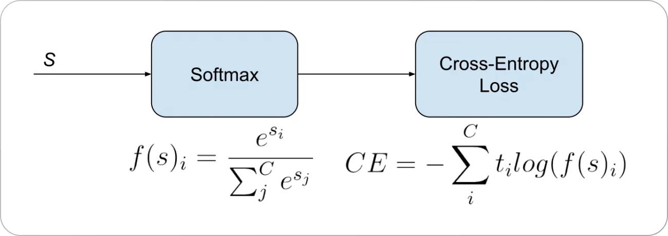
Cross-entropy loss formula (source)

The image below shows the workflow of image classification inference:

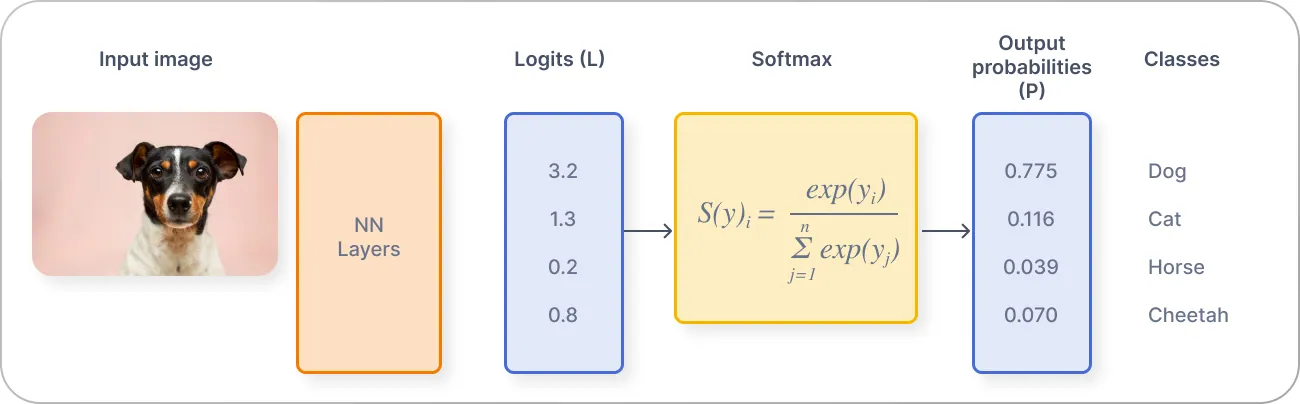
Image classification using cross-entropy loss (S is Softmax output, T—target) (source)

Softmax converts logits into probabilities. The purpose of cross-entropy is to take the output probabilities (P) and measure the distance from the truth values (as shown below).

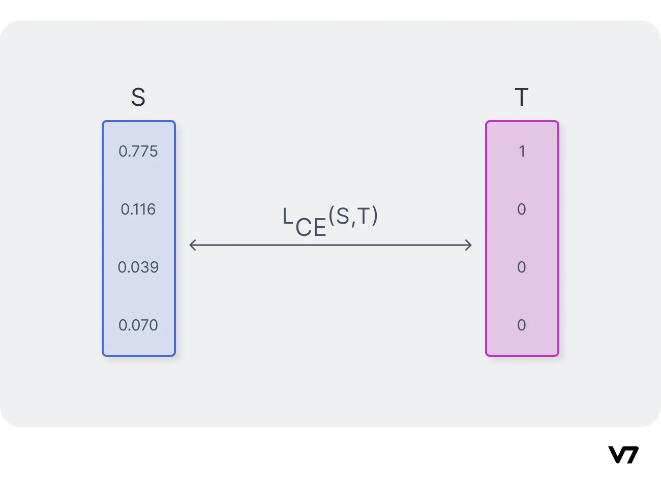
Cross Entropy (L) (S is Softmax output, T — target)

The image below illustrates the input parameter to the cross entropy loss function:

Cross-entropy loss parameters

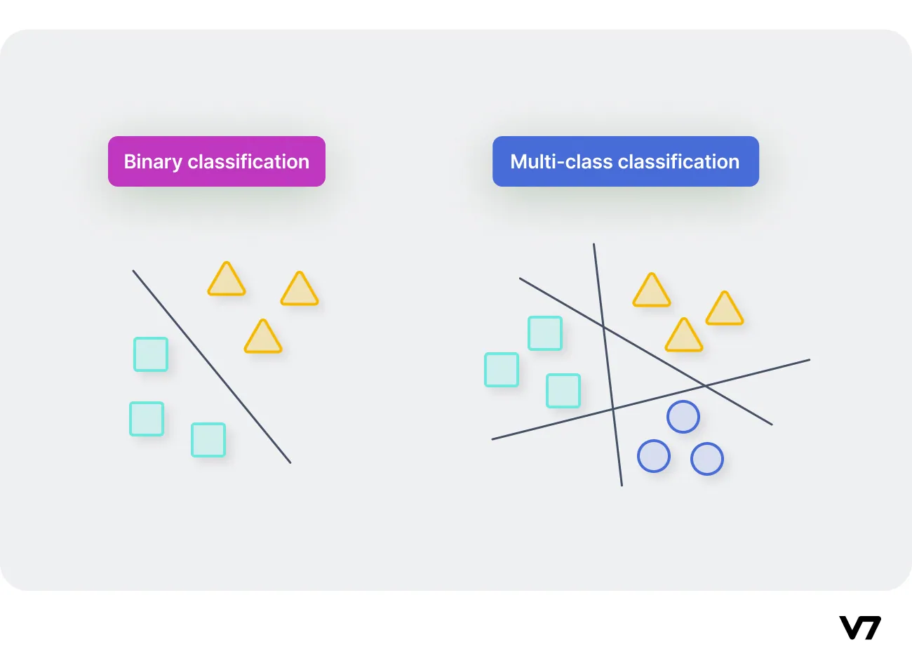
Binary cross-entropy loss

Binary cross entropy is the loss function used for classification problems between two categories only. It’s also known as a binary classification problem.

The Probability Mass Function (PMF) is used (return probability) when dealing with discrete quantities. For continuous values where Mean Squared Error is used, Probability Density Function (PDF) (return density) is applied instead.

PMF used in this function is represented by the following equation:

PMF for binary cross entropy

Here, the x is constant because it is present in the data, and mu is the variable.

To maximize the likelihood, PMF can be represented as:

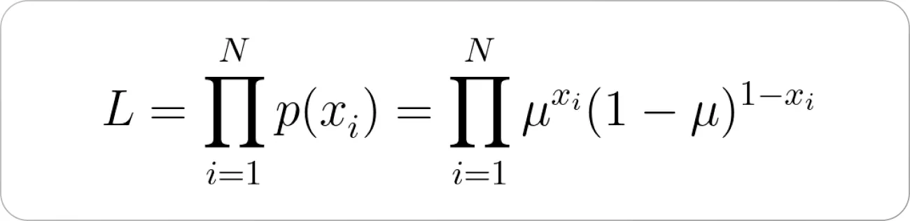
Log likelihood equation using PMF

To perform the calculations, take the log of this function, as it allows us to minimize/maximize using derivatives quickly. Taking the log before processing is allowed because the log is a monotonically increasing function.

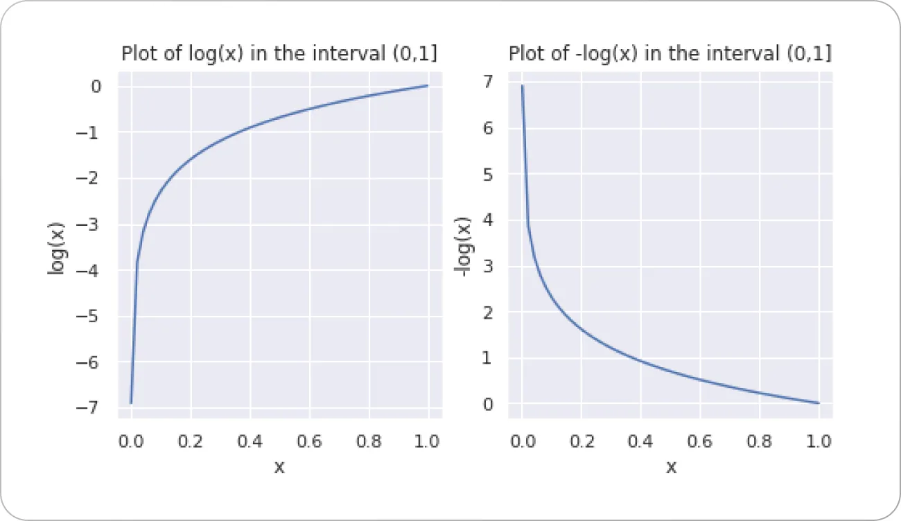
Logarithmic function range

As seen in the plots above, in the interval (0,1], log(x) and -log(x) are negative and positive, respectively. Observe how -log(x) approaches 0 as x approaches 1. This observation is useful when parsing the expression for cross-entropy loss.

Since we want to maximize the probability of the output falling into a specific category, the mu value has to be found in the below log-likelihood equation.

Log likelihood

Calculate the partial derivative of the above log-likelihood function with respect to mu. The output is:

Mean over probabilities of n samples in the dataset

In the above equation, x(i) will have a probability value of either 1 or 0.

Let’s take the coin toss as an example. If we are looking for heads, the value of x()

For example, in the coin toss, if we are looking for heads, if a head appears, then the value of x(i) will be 1; otherwise, 0. This way, the above equation will calculate the probability of the desired outcome in all the events.

If we maximize the likelihood or minimize the negative log-likelihood (it is the actual error in prediction and actual value), the outcome is the same

Therefore the negative log-likelihood will be:

Negative log likelihood formula

In the negative log-likelihood equation, mu will become y_pred—the class corresponding to maximum probability of i (class into which y(i) is classified based on the maximum probability).

If there are n samples in the dataset, then the total cross-entropy loss is the sum of the loss values over all the samples in the dataset. So the binary cross entropy (BCE) to minimize the error can be formulated in the following way:

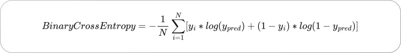
Binary cross entropy formula

Binary cross entropy loss function w.r.t to p value (source)

From the calculations above, we can make the following observations:

When the true label t is 1, the cross-entropy loss approaches 0 as the predicted probability p approaches 1 and
When the true label t is 0, the cross-entropy loss approaches 0 as the predicted probability p approaches 0.

Multi-class cross-entropy/categorical cross-entropy

Multi-class classification

Categorical Cross Entropy is also known as Softmax Loss. It’s a softmax activation plus a Cross-Entropy loss used for multiclass classification. Using this loss, we can train a Convolutional Neural Network to output a probability over the N classes for each image.

In multiclass classification, the raw outputs of the neural network are passed through the softmax activation, which then outputs a vector of predicted probabilities over the input classes.

In the specific (and usual) case of multi-class classification, the labels are one-hot, so only the positive class keeps its term in the loss. There is only one element of the target vector, different than zero. Discarding the elements of the summation which are zero due to target labels, we can write:

Binary classification vs. Multi-class classification

A video labeling annotation tool where drone footage of a port inspection is being annotated

Video annotation

AI video annotation

Get started today

Video annotation

AI video annotation

Get started today

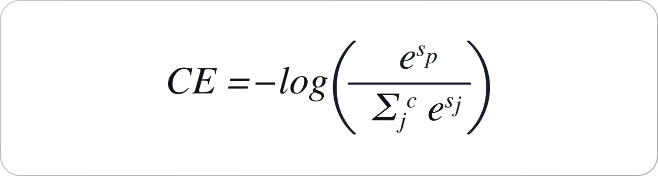
Categorical cross-entropy loss forward function in Python

def forward(self, bottom, top):
  labels = bottom[1].data
  scores = bottom[0].data
  # Normalizing to avoid instability
  scores -= np.max(scores, axis=1, keepdims=True) 
  # Compute Softmax activations
  exp_scores = np.exp(scores)
  probs = exp_scores / np.sum(exp_scores, axis=1, keepdims=True)
  logprobs = np.zeros([bottom[0].num,1])
  # Compute cross-entropy loss
  for r in range(bottom[0].num): # For each element in the batch
      scale_factor = 1 / float(np.count_nonzero(labels[r, :]))
      for c in range(len(labels[r,:])): # For each class
          if labels[r,c] != 0:  # Positive classes
              logprobs[r] += -np.log(probs[r,c]) * labels[r,c] * scale_factor # We sum the loss per class for each element of the batch


  data_loss = np.sum(logprobs) / bottom[0].num


  self.diff[...] = probs  # Store softmax activations
  top[0].data[...] = data_loss # Store loss

Categorical cross-entropy vs. sparse categorical cross-entropy

The loss function for categorical cross entropy and sparse categorical cross entropy is the same, and it differs in the way you mention Yi (i,e accurate labels).

Categorical Cross Entropy

Labels (Yi) are one-hot encoded.

Examples (for a 3-class classification): [1,0,0] , [0,1,0], [0,0,1]

Sparse Categorical Cross Entropy

Labels (Yi) are integers.

Examples of the above 3-class classification problem: [1], [2], [3]

Moreover, it depends on how you load the dataset. Loading the dataset labels using integers instead of vectors provides greater memory and computation efficiency.

Coding cross-entropy in Pytorch and Tensorflow

Not that we covered the fundamentals of Cross Entropy, let’s jump right into the code.

PyTorch

Define a dummy input and target to test the cross entropy loss pytorch function.
Import CrossEntropyLoss() inbuilt function from torch.nn module.
Define the loss variable and pass the inputs and target
Call the output backward function to compute gradients to improve loss in the next training iteration.

z# Example of target with class probabilities
import torch
import torch.nn as nn


input = torch.rand(3, 5, requires_grad=True)
target = torch.empty(3, dtype=torch.long).random_(5)
print(target.size())
loss = nn.CrossEntropyLoss()
output = loss(input, target)
output.backward()
print("Input:",input)
print("Target:",target)
print("Cross Entropy Loss:",output)
print('Input grads: ', input.grad)

torch.Size([3])
Input:
  tensor([[0.8671, 0.0189, 0.0042, 0.1619, 0.9805],
     [0.1054, 0.1519, 0.6359, 0.6112, 0.9417],
     [0.9968, 0.3285, 0.9185, 0.0315, 0.9592]],
     requires_grad=True)
Target:
  tensor([1, 0, 4])
Cross Entropy Loss:
  tensor(1.8338, grad_fn=<NllLossBackward>

In this example, we only considered a single training sample. In reality, we usually do mini-batches. By default, PyTorch will use the average cross-entropy loss of all samples in the batch.

In Pytorch, if one uses the nn.CrossEntropyLoss, the input must be an unnormalized raw value (logits), and the target must be a class index instead of one hot encoded vector.

Binary cross entropy is a case where the number of classes is 2. In PyTorch, there are nn.BCELoss and nn.BCEWithLogitsLoss. The former requires the input normalized sigmoid probability, an the latter can take raw unnormalized logits.

See Pytorch documentation on CrossEntropyLoss.

Tensorflow

Define a dummy input and target to test TensorFlow's cross-entropy loss function.
Import BinaryCrossentropy() inbuilt function from tf.keras.losses module.
Define loss variable binary_cross_entropy and pass the inputs and target.
Call the output backward function to compute gradients to improve loss in the following training iteration.

## Binary Cross Entropy Calculation
import tensorflow as tf


#input lables.
y_true = [[0.,1.],
        [0.,0.]]
y_pred = [[0.5,0.4],
        [0.6,0.3]]


binary_cross_entropy = tf.keras.losses.BinaryCrossentropy()
binary_cross_entropy(y_true=y_true,y_pred=y_pred).numpy()

Key takeaways

Here’s a short recap of what we’ve learned about cross-entropy loss.

Entropy is a measure of uncertainty, i.e., if an outcome is certain, entropy is low.
Cross-entropy loss, or log loss, measures the performance of a classification model whose output is a probability value between 0 and 1. Cross-entropy loss increases as the predicted probability diverges from the actual label.
Binary cross entropy is calculated on top of sigmoid outputs, whereas Categorical cross-entropy is calculated over softmax activation outputs.
Categorical cross-entropy is used for multi-class classification.
Cross-entropy is different from KL divergence but can be calculated using KL divergence. It’s also different from log loss but calculates the same quantity when used as a machine learning loss function.

Next steps

Label videos with V7.

Rewind less, achieve more.

Try our free tier or talk to one of our experts.

Next steps

Label videos with V7.

Rewind less, achieve more.